对“教你使用简单神经网络和LSTM进行时间序列预测”代码修改与解读

原文链接和代码在这里：教你使用简单神经网络和LSTM进行时间序列预测（附代码）

但是在测试的过程中，原代码出现一些问题，直接运行原文中的代码是行不通的。大部分的代码解释原文写的很明白，这里只做补充。

本文测试环境：Python3.6  Jupyter Notebook，TensorFlow+Keras

这篇文章采用人工神经网络（Artificial Neural Network ，ANN）和长短期记忆循环神经网络（Long Short-Term Memory Recurrent Neural Network ，LSTM RNN）对时间序列数据建立模型，目标是采用ANN和LSTM来预测波动性标准普尔500时间序列。

可以从这里（https://ca.finance.yahoo.com/quote/%5Evix/history?ltr=1）下载波动性标准普尔500数据集,可以选择你要下载的数据集的时间范围。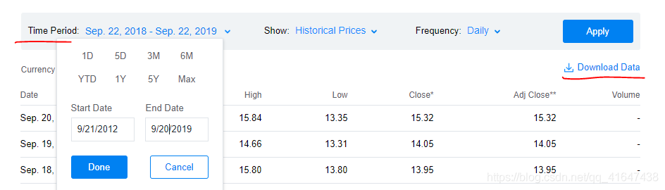

开始敲代码吧。首先是ANN模型

import pandas as pd
import numpy as np
%matplotlib inline 
#在Jupyter Notebook要PLOT出图像，必须加这个
import matplotlib.pyplot as plt
from sklearn.preprocessing import MinMaxScaler
from sklearn.metrics import r2_score
from keras.models import Sequential
from keras.layers import Dense
from keras.callbacks import EarlyStopping
from keras.optimizers import Adam
from keras.layers import LSTM
#并将数据加载到Pandas 的dataframe中。
df = pd.read_csv("E:\data\VIX.csv")
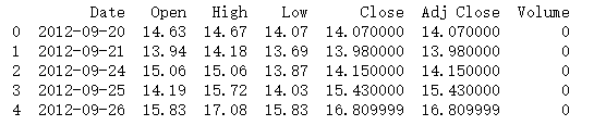
#我们可以快速浏览前几行。
print(df.head())
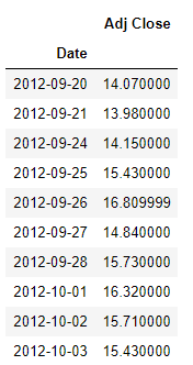
#删除不需要的列，然后将“日期”列转换为时间数据类型，并将“日期”列设置为索引。
df.drop(['Open', 'High', 'Low', 'Close', 'Volume'], axis=1, inplace=True)
df['Date'] = pd.to_datetime(df['Date'])
df = df.set_index(['Date'], drop=True)
df.head(10)

Out[1]:

Out[2]:

(我们只用Adj Close这个数据)

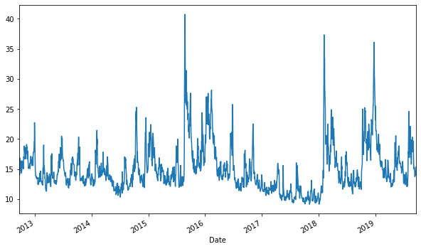
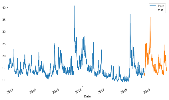
#我们绘制一个时间序列线图。
plt.figure(figsize=(10, 6))
df['Adj Close'].plot();

#按日期“2018–09–20”将数据拆分为训练集和测试集
split_date = pd.Timestamp('2018-09-20')
df = df['Adj Close']
train = df.loc[:split_date]
test = df.loc[split_date:]
plt.figure(figsize=(10, 6))
ax = train.plot()
test.plot(ax=ax)
plt.legend(['train', 'test']);

Out:

#将训练和测试数据缩放为[-1，1]。
train=np.array(train).reshape(-1,1)
test=np.array(test).reshape(-1,1)

scaler = MinMaxScaler(feature_range=(-1, 1))
train_sc = scaler.fit_transform(train)
test_sc = scaler.fit_transform(test)

对之前的归一化还原：

origin_data=scaler.inverse_transform(y_pred_test)‘‘’

最后会加上对数据还原的部分

#获取训练和测试数据。
X_train = train_sc[:-1]
y_train = train_sc[1:]
X_test = test_sc[:-1]
y_test = test_sc[1:]
#获取训练和测试数据。
X_train = train_sc[:-1]
y_train = train_sc[1:]
X_test = test_sc[:-1]
y_test = test_sc[1:]

解释，序列预测a=np.array([2,3,4,5,6,7])

print(a[:-1]) #去掉最后一个元素

print(a[1:]) #从第二个元素开始

Out:

[2 3 4 5 6]

[3 4 5 6 7]

输入x=[2 3 4 5 6]

对应的Label y=[3 4 5 6 7]  (递进预测下一个)‘‘’

#用于时间序列预测的简单人工神经网络ANN
ann=Sequential()
ann.add(Dense(12, input_dim=1, activation='relu'))
ann.add(Dense(1))
ann.compile(loss='mean_squared_error', optimizer='adam')
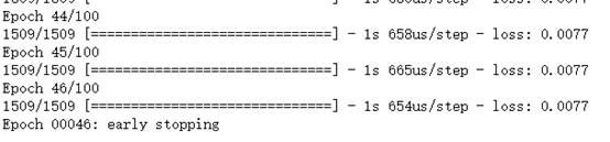
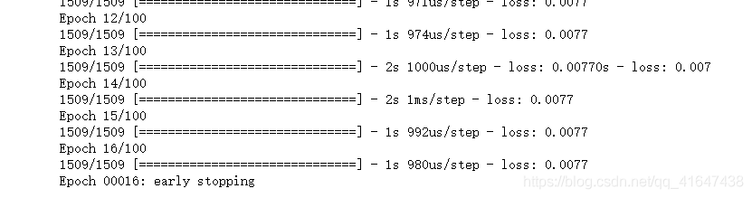
early_stop = EarlyStopping(monitor='loss', patience=2, verbose=1)
history= ann.fit(X_train, y_train, epochs=100, batch_size=1, verbose=1, callbacks=[early_stop], shuffle=False)

#进行预测
y_pred_test = ann.predict(X_test)

y_train_pred =ann.predict(X_train)

print("The R2 score on the Train set is:\t{:0.3f}".format(r2_score(y_train, y_train_pred)))

print("The R2 score on the Test set is:\t{:0.3f}".format(r2_score(y_test, y_pred_test)))

Out:

The R2 score on the Train set is:     0.851

The R2 score on the Test set is:      0.823

补充：

R2 决定系数（拟合优度）

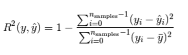
模型越好：r2→1

模型越差：r2→0

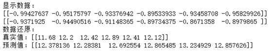
#显示6项数据
print('显示数据：')
print(y_test[:6].reshape([1,6]))
print(y_pred_test[:6].reshape([1,6]))
#将归一化数据还原
y_test_pred_origin=scaler.inverse_transform(y_pred_test)
y_test_origin=scaler.inverse_transform(y_test)
print('数据还原：')
print('真实值：'+'%s'%y_test_origin[:6].reshape([1,6]))
print('预测值：'+'%s'%y_test_pred_origin[:6].reshape([1,6]))

Out:  （后面有预测和真实的评估指标MSE）

 

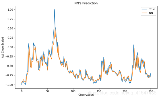
#显示TEST真实值和预测值的对比图
plt.figure(figsize=(10, 6))

plt.plot(y_test, label='True')

plt.plot(y_pred_test, label='NN')

plt.title("NN's Prediction")

plt.xlabel('Observation')

plt.ylabel('Adj Close Scaled')

plt.legend()

plt.show();

OUT:

LSTM 模型

x_train=X_train.reshape(1509,1,1)#注意input x_train 的shape
lstm_model = Sequential()
lstm_model.add(LSTM(7,activation='relu', kernel_initializer='lecun_uniform', return_sequences=False))
lstm_model.add(Dense(1))
lstm_model.compile(loss='mean_squared_error', optimizer='adam')
early_stop = EarlyStopping(monitor='loss', patience=2, verbose=1)
history_lstm_model = lstm_model.fit(x_train, y_train, epochs=100, batch_size=1, verbose=1, shuffle=False, callbacks=[early_stop])

LSTM模型输入的shape和ANN有差别，所以要先对X_train 进行变换，后面的X_test也是如此。

OUT:

进行预测

x_test=X_test.reshape(251,1,1) #251 is the length of X_test
y_pred_test_lstm = lstm_model.predict(x_test)
y_train_pred_lstm = lstm_model.predict(x_train)
print("The R2 score on the Train set is:t{:0.3f}".format(r2_score(y_train, y_train_pred_lstm)))
print("The R2 score on the Test set is:t{:0.3f}".format(r2_score(y_test, y_pred_test_lstm)))

OUT:

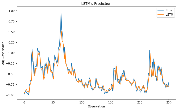
#显示TEST真实值和预测值的对比图
plt.figure(figsize=(10, 6))
plt.plot(y_test, label='True')
plt.plot(y_pred_test_lstm, label='LSTM')
plt.title("LSTM's Prediction")
plt.xlabel('Observation')
plt.ylabel('Adj Close scaled')
plt.legend()
plt.show()

OUT:

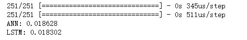
#比较了两种模型的测试MSE
ann_test_mse = ann.evaluate(X_test, y_test, batch_size=1)
lstm_test_mse = lstm_model.evaluate(x_test, y_test, batch_size=1)
print('ANN: %f'%ann_test_mse)
print('LSTM: %f'%lstm_test_mse)

Out:

小结：

其实要修改的地方不是很多，这是一个比较简单的例子，不熟悉的话可能会费时间，对numpy和pandas要多加学习和练习。