传统车道线检测
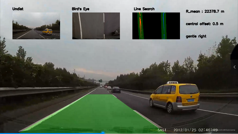
Advanced_Lane_Detection项目的复现,更换了其中的数据,修改了相应脚本,添加了可视化功能。话不多说,直接上图显示效果。
文章目录
环境要求
- Python 3.5
- Numpy
- OpenCV-Python
- Matplotlib
- Pickle
项目流程
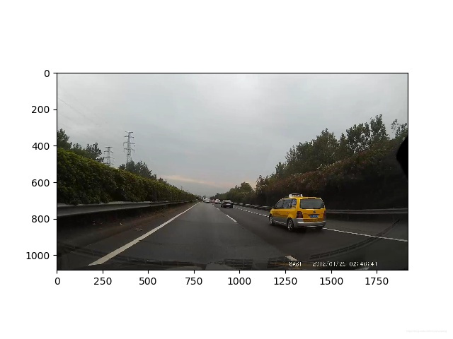
一:相机标定
采用棋盘格对相机进行标定,消除畸变,可采用下列方法(本项目采用第二种)
- 法一:执行calibrate_camera.py脚本获得内参矩阵与畸变系数存入p文件
def calibrate_camera():
	# 棋盘格个数及其横纵内角点个数
	objp_dict = {
		1: (9, 6),
		2: (9, 6),
		3: (9, 6),
		4: (9, 6),
		5: (9, 6),
		6: (9, 6),
		7: (9, 6),
		8: (9, 6),
		9: (9, 6),
		10: (9, 6),
		11: (9, 6),
		12: (9, 6),
		13: (9, 6),
		14: (9, 6),
		15: (9, 6),
		16: (9, 6),
		17: (9, 6),
		18: (9, 6),
		19: (9, 6),
		20: (9, 6),
	}

	objp_list = []
	corners_list = []

	for k in objp_dict:
		nx, ny = objp_dict[k]
		objp = np.zeros((nx*ny,3), np.float32)
		objp[:,:2] = np.mgrid[0:nx, 0:ny].T.reshape(-1,2)
		fname = 'camera_cal/calibration%s.jpg' % str(k)
		img = cv2.imread(fname)
		gray = cv2.cvtColor(img, cv2.COLOR_BGR2GRAY)
		# 棋盘格角点
		ret, corners = cv2.findChessboardCorners(gray, (nx, ny), None)

		if ret == True:
			objp_list.append(objp)
			corners_list.append(corners)
		else:
			print('Warning: ret = %s for %s' % (ret, fname))

	# 相机标定
	img = cv2.imread('test_images/straight_lines1.jpg')
	img_size = (img.shape[1], img.shape[0])
	ret, mtx, dist, rvecs, tvecs = cv2.calibrateCamera(objp_list, corners_list, img_size,None,None)

	return mtx, dist
- 法二:借助Matlab相机标定工具包,傻瓜式操作得到内参矩阵与畸变系数存入p文件
具体操作请看Matlab相机标定
二:ROI操作
设置mask,只保留车辆前方ROI区域,以便减小二值化处理的难度
def region_of_interest(img, vertices):
    mask = np.zeros_like(img)
    if len(img.shape) > 2:
        channel_count = img.shape[2]
        ignore_mask_color = (255,) * channel_count
    else:
        ignore_mask_color = 255
    cv2.fillPoly(mask, vertices, ignore_mask_color)
    masked_image = cv2.bitwise_and(img, mask)

    return masked_image
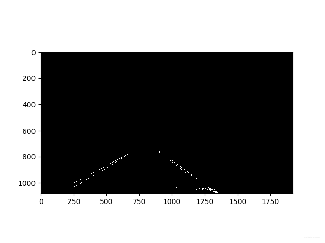
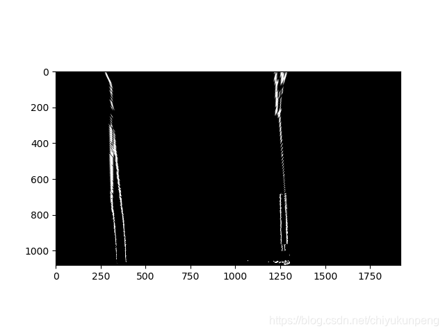
三:二值化操作
基于图像的梯度和颜色信息,进行二值化处理,阈值自行调整,初步定位车道线所在位置
# SobelX,SobelY梯度信息
def abs_sobel_thresh(img, orient='x', thresh_min=20, thresh_max=100):
	gray = cv2.cvtColor(img, cv2.COLOR_RGB2GRAY)
	if orient == 'x':
		abs_sobel = np.absolute(cv2.Sobel(gray, cv2.CV_64F, 1, 0))
	if orient == 'y':
		abs_sobel = np.absolute(cv2.Sobel(gray, cv2.CV_64F, 0, 1))

	scaled_sobel = np.uint8(255*abs_sobel/np.max(abs_sobel))
	binary_output = np.zeros_like(scaled_sobel)
	binary_output[(scaled_sobel >= thresh_min) & (scaled_sobel <= thresh_max)] = 1

	return binary_output

# SobelXY梯度信息
def mag_thresh(img, sobel_kernel=3, mag_thresh=(30, 100)):
	gray = cv2.cvtColor(img, cv2.COLOR_RGB2GRAY)
	sobelx = cv2.Sobel(gray, cv2.CV_64F, 1, 0, ksize=sobel_kernel)
	sobely = cv2.Sobel(gray, cv2.CV_64F, 0, 1, ksize=sobel_kernel)
	gradmag = np.sqrt(sobelx**2 + sobely**2)
	scale_factor = np.max(gradmag)/255
	gradmag = (gradmag/scale_factor).astype(np.uint8)
	binary_output = np.zeros_like(gradmag)
	binary_output[(gradmag >= mag_thresh[0]) & (gradmag <= mag_thresh[1])] = 1

	return binary_output

# direction信息
def dir_threshold(img, sobel_kernel=3, thresh=(0, np.pi/2)):
	gray = cv2.cvtColor(img, cv2.COLOR_RGB2GRAY)
	sobelx = cv2.Sobel(gray, cv2.CV_64F, 1, 0, ksize=sobel_kernel)
	sobely = cv2.Sobel(gray, cv2.CV_64F, 0, 1, ksize=sobel_kernel)
	absgraddir = np.arctan2(np.absolute(sobely), np.absolute(sobelx))
	binary_output =  np.zeros_like(absgraddir)
	binary_output[(absgraddir >= thresh[0]) & (absgraddir <= thresh[1])] = 1

	return binary_output

# S通道信息
def hls_thresh(img, thresh=(100, 255)):
	hls = cv2.cvtColor(img, cv2.COLOR_RGB2HLS)
	s_channel = hls[:,:,2]
	binary_output = np.zeros_like(s_channel)
	binary_output[(s_channel > thresh[0]) & (s_channel <= thresh[1])] = 1

	return binary_output

# 叠加信息,四组阈值可以适当调整
def combined_thresh(img):
	abs_bin = abs_sobel_thresh(img, orient='x', thresh_min=35, thresh_max=100)
	mag_bin = mag_thresh(img, sobel_kernel=3, mag_thresh=(30, 255))
	dir_bin = dir_threshold(img, sobel_kernel=15, thresh=(0.7, 1.3))
	hls_bin = hls_thresh(img, thresh=(80, 255))

	combined = np.zeros_like(dir_bin)
	combined[(abs_bin == 1 | ((mag_bin == 1) & (dir_bin == 1))) | hls_bin == 1] = 1

	return combined, abs_bin, mag_bin, dir_bin, hls_bin
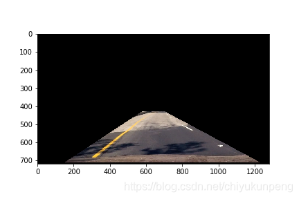
四:透视变换
运用透视变换,将二值图像转换为鸟瞰图,其中源点与目标点坐标的设置非常重要,以便后期使用多项式拟合进一步精准检测车道线
def perspective_transform(img):
	img_size = (img.shape[1], img.shape[0])

    # 源点(左下,左上,右上,右下)
	src = np.float32([[310, 1080],[750, 760],[910, 760],[1370, 1080]])
	# 目标点(左下,左上,右上,右下)
	dst = np.float32([[500,1080],[500,0],[1300,0], [1300,1080]])

	# 透射变换矩阵,逆透视变换矩阵
	m = cv2.getPerspectiveTransform(src, dst)
	m_inv = cv2.getPerspectiveTransform(dst, src)

	warped = cv2.warpPerspective(img, m, img_size, flags=cv2.INTER_LINEAR)
	unwarped = cv2.warpPerspective(warped, m_inv, (warped.shape[1], warped.shape[0]), flags=cv2.INTER_LINEAR)

	return warped, unwarped, m, m_inv
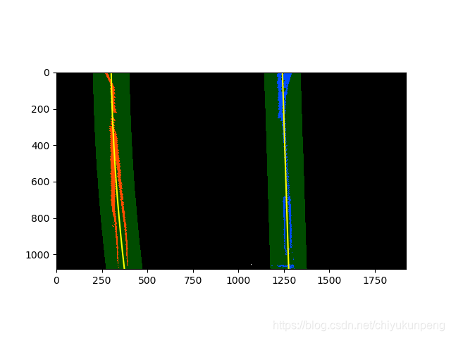
五:多项式拟合
- 直方图统计,定位峰值为左右车道线搜寻基点
- 运用滑窗检测车道线,滑窗的数目,大小,面积设置可调
- 多项式方程 ayy+by+c=x 不断得到新的搜寻基点
- 可视化操作
# 车道线拟合
def line_fit(binary_warped):
	# 直方图
	histogram = np.sum(binary_warped[binary_warped.shape[0]//2:,:], axis=0)
	out_img = (np.dstack((binary_warped, binary_warped, binary_warped))*255).astype('uint8')
	midpoint = np.int(histogram.shape[0]/2)
	leftx_base = np.argmax(histogram[100:midpoint]) + 100
	rightx_base = np.argmax(histogram[midpoint:-100]) + midpoint

	# 滑窗数目
	nwindows = 9
	window_height = np.int(binary_warped.shape[0]/nwindows)
	nonzero = binary_warped.nonzero()
	nonzeroy = np.array(nonzero[0])
	nonzerox = np.array(nonzero[1])
	leftx_current = leftx_base
	rightx_current = rightx_base
	# 滑窗宽度允许变动阈值
	margin = 100
	# 滑窗面积阈值
	minpix = 50

	left_lane_inds = []
	right_lane_inds = []

	for window in range(nwindows):
		win_y_low = binary_warped.shape[0] - (window+1)*window_height
		win_y_high = binary_warped.shape[0] - window*window_height

		win_xleft_low = leftx_current - margin
		win_xleft_high = leftx_current + margin
		win_xright_low = rightx_current - margin
		win_xright_high = rightx_current + margin

		cv2.rectangle(out_img,(win_xleft_low,win_y_low),(win_xleft_high,win_y_high),(0,255,0), 2)
		cv2.rectangle(out_img,(win_xright_low,win_y_low),(win_xright_high,win_y_high),(0,255,0), 2)

		good_left_inds = ((nonzeroy >= win_y_low) & (nonzeroy < win_y_high) & (nonzerox >= win_xleft_low) & (nonzerox < win_xleft_high)).nonzero()[0]
		good_right_inds = ((nonzeroy >= win_y_low) & (nonzeroy < win_y_high) & (nonzerox >= win_xright_low) & (nonzerox < win_xright_high)).nonzero()[0]

		left_lane_inds.append(good_left_inds)
		right_lane_inds.append(good_right_inds)

		if len(good_left_inds) > minpix:
			leftx_current = np.int(np.mean(nonzerox[good_left_inds]))
		if len(good_right_inds) > minpix:
			rightx_current = np.int(np.mean(nonzerox[good_right_inds]))

	left_lane_inds = np.concatenate(left_lane_inds)
	right_lane_inds = np.concatenate(right_lane_inds)

	leftx = nonzerox[left_lane_inds]
	lefty = nonzeroy[left_lane_inds]
	rightx = nonzerox[right_lane_inds]
	righty = nonzeroy[right_lane_inds]

	left_fit = np.polyfit(lefty, leftx, 2)
	right_fit = np.polyfit(righty, rightx, 2)

	ret = {}
	ret['left_fit'] = left_fit
	ret['right_fit'] = right_fit
	ret['nonzerox'] = nonzerox
	ret['nonzeroy'] = nonzeroy
	ret['out_img'] = out_img
	ret['left_lane_inds'] = left_lane_inds
	ret['right_lane_inds'] = right_lane_inds

	return ret
六:计算曲率半径与车辆中心距车道中心偏移量
借助像素与米的换算关系,可求出曲率半径以及车辆中心距车道中心偏移量,进而给出车辆状态
# 计算曲率半径
def calc_curve(left_lane_inds, right_lane_inds, nonzerox, nonzeroy):
	# 图片高度最大值索引
	y_eval = 1079

	# 图片单位像素与米的换算关系
	xm_per_pix = 3.75 / 1100
	ym_per_pix = 30 / 720

	leftx = nonzerox[left_lane_inds]
	lefty = nonzeroy[left_lane_inds]
	rightx = nonzerox[right_lane_inds]
	righty = nonzeroy[right_lane_inds]

	left_fit_cr = np.polyfit(lefty*ym_per_pix, leftx*xm_per_pix, 2)
	right_fit_cr = np.polyfit(righty*ym_per_pix, rightx*xm_per_pix, 2)

	left_curverad = ((1 + (2*left_fit_cr[0]*y_eval*ym_per_pix + left_fit_cr[1])**2)**1.5) / np.absolute(2*left_fit_cr[0])
	right_curverad = ((1 + (2*right_fit_cr[0]*y_eval*ym_per_pix + right_fit_cr[1])**2)**1.5) / np.absolute(2*right_fit_cr[0])

	return left_curverad, right_curverad

# 计算距车道中心偏移量
def calc_vehicle_offset(undist, left_fit, right_fit):
	bottom_y = undist.shape[0] - 1
	bottom_x_left = left_fit[0]*(bottom_y**2) + left_fit[1]*bottom_y + left_fit[2]
	bottom_x_right = right_fit[0]*(bottom_y**2) + right_fit[1]*bottom_y + right_fit[2]
	vehicle_offset = undist.shape[1]/2 - (bottom_x_left + bottom_x_right)/2
	# 图片单位像素与米的换算关系
	xm_per_pix = 3.75/1100
	vehicle_offset *= xm_per_pix

	return vehicle_offset
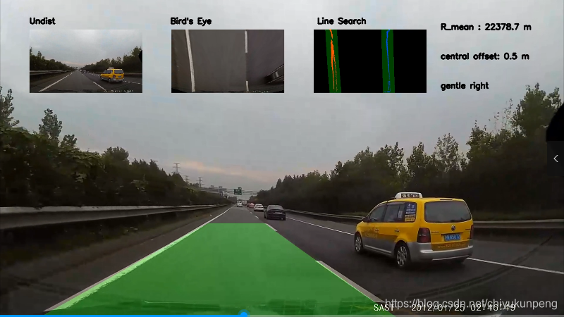
七:可视化
在视频上方分别实时显示消除畸变的图片,鸟瞰图片,多项式拟合图片以及曲率半径,车辆中心距车道中心偏移量
def final_viz(undist, left_fit, right_fit, m_inv, left_curve, right_curve, vehicle_offset):
	ploty = np.linspace(0, undist.shape[0]-1, undist.shape[0])
	left_fitx = left_fit[0]*ploty**2 + left_fit[1]*ploty + left_fit[2]
	right_fitx = right_fit[0]*ploty**2 + right_fit[1]*ploty + right_fit[2]

	# 创建图片
	color_warp = np.zeros((1080, 1920, 3), dtype='uint8')

	pts_left = np.array([np.transpose(np.vstack([left_fitx, ploty]))])
	pts_right = np.array([np.flipud(np.transpose(np.vstack([right_fitx, ploty])))])
	pts = np.hstack((pts_left, pts_right))

	cv2.fillPoly(color_warp, np.int_([pts]), (0,255, 0))

	newwarp = cv2.warpPerspective(color_warp, m_inv, (undist.shape[1], undist.shape[0]))
	result = cv2.addWeighted(undist, 1, newwarp, 0.3, 0)

	# 图片右上角显示曲率半径,中心偏移量
	avg_curve = (left_curve + right_curve)/2
	string1 = 'R_mean : %.1f m' % avg_curve
	if left_fit[0] > 0 and avg_curve > 500:
		string2 = "gentle right"
	elif left_fit[0] > 0 and avg_curve <= 500:
		string2 = "hard right"
	elif left_fit[0] < 0 and avg_curve > 500:
		string2 = "gentle left"
	elif left_fit[0] < 0 and avg_curve <= 500:
		string2 = "hard left"
	string3 = 'central offset: %.1f m' % vehicle_offset

	font = cv2.FONT_HERSHEY_SIMPLEX
	cv2.putText(result, string1, (1500, 100), font, 0.9, (0, 0, 0), 4, cv2.LINE_AA)
	cv2.putText(result, string2, (1500, 300), font, 0.9, (0, 0, 0), 4, cv2.LINE_AA)
	cv2.putText(result, string3, (1500, 200), font, 0.9, (0, 0, 0), 4, cv2.LINE_AA)

	# 图片上方显示消除失真图,鸟瞰图,车道线检测图
	small_undist = cv2.resize(undist, (0, 0), fx=0.2, fy=0.2)
	bird_eye, _, _, _ = perspective_transform(undist)
	small_bird_eye = cv2.resize(bird_eye, (0, 0), fx=0.2, fy=0.2)

	img = cv2.cvtColor(undist, cv2.COLOR_BGR2RGB)
	vertices = np.int32([[(50, 1080), (700, 760), (920, 760), (1400, 1080)]])
	masked_image = region_of_interest(img, vertices)
	cv2.line(masked_image, (50, 1080), (700, 760), (0, 0, 0), 10)
	cv2.line(masked_image, (920, 760), (1400, 1080), (0, 0, 0), 25)
	img, abs_bin, mag_bin, dir_bin, hls_bin = combined_thresh(masked_image)
	binary_warped, binary_unwarped, m, m_inv = perspective_transform(img)
	ret = line_fit(binary_warped)
	out_image = viz2(binary_warped, ret)
	small_out_image = cv2.resize(out_image, (0, 0), fx=0.2, fy=0.2)

	x1 = 0
	y1 = 100
	x2 = small_out_image.shape[0]
	y2 = small_out_image.shape[1]
	y3 = small_out_image.shape[1] * 2
	y4 = small_out_image.shape[1] * 3
	result[x1 + 100:x2 + 100, y1:y2 + 100, :] = small_undist
	result[x1 + 100:x2 + 100, y2 + 200:y3 + 200, :] = small_bird_eye
	result[x1 + 100:x2 + 100, y3 + 300:y4 + 300, :] = small_out_image
	cv2.putText(result, "Undist", (100, 80), font, 0.9, (0, 0, 0), 4, cv2.LINE_AA)
	cv2.putText(result, "Bird's Eye", (580, 80), font, 0.9, (0, 0, 0), 4, cv2.LINE_AA)
	cv2.putText(result, "Line Search", (1080, 80), font, 0.9, (0, 0, 0), 4, cv2.LINE_AA)

	return result
总结与展望
总结
- 传统图像处理算法检测车道线受外界因素影响较大,精度一般
- 这个项目的bug在于车道线检测偶尔不准,后期曲率半径的计算会失准,但车辆中心距车道中心的偏移量准确
- 透视变换对于车道线检测精度提升有很大帮助
展望
- 利用偏移量可进一步实现自动修正方位功能
- 透视变换对于遮挡这一因素的消除十分有效,可应用到其他场合
附:
鸣谢
- 特别鸣谢视觉测控与智能导航实验室泽阳大神,附上大神Github主页链接
- 鸣谢临港六狼团队所有成员以及张老板的大力指导
