TensorFlow 2官方教程 . Keras机器学习基础知识 . 基本图像分类

写在前面

此篇博客翻译自tensorflow官方教程:
https://www.tensorflow.org/tutorials/keras/classification
笔者吐槽一下: 本来只打算转载顺便看看官方教程，结果这一篇的前后两篇都翻译了，它却没被翻译
另外，笔者水平有限，若有翻译错误，还请不吝赐教，同时笔者会以注释的形式将可能由环境问题带来的BUG写出来
如果之后该文档被翻译了，还请小伙伴们通知我一下

此博客教程可在tensorflow官方github 上下载：
https://github.com/tensorflow/docs/blob/master/site/en/tutorials/keras/classification.ipynb

---

简单衣物图像分类(Basic classification: Classify images of clothing)

本教程将教你，训练一个能将简单衣物进行分类的神经网络。即使你不懂得所有细节那也是很OK的，因为，本教程将带你快速了解写tensorflow程序的全过程，随着你的阅读，你将了解到一些神经网络的细节。

这篇教程使用tf.keras，这是一个在Tensorflow中高级API，主要用来建立和训练模型。

from __future__ import absolute_import, division, print_function, unicode_literals

# 导入 TensorFlow 和 tf.keras
import tensorflow as tf[添加链接描述](https://github.com/zalandoresearch/fashion-mnist)
from tensorflow import keras

# 导入 numpy 和 matplotlib
import numpy as np
import matplotlib.pyplot as plt

1.导入我们经典的数据集——Fashion MNIST

Fashion MNIST数据集有10类图片，总共70000张灰度图片。每张图片以（28 x 28像素）的低分辨率显示单件衣服，如下所示：

↑Figure1. Fashion-MNIST样本(by Zalando, MIT License)↑

---

• Fashion MNIST数据集旨在替代经典MNIST数据集，而MNIST数据集就是小白接触计算机视觉机器学习程序的HelloWorld。
• Fashion MNIST数据集中衣服图片数据的格式与MNIST数据集中手写数字图片的格式相同。
• 本教程将Fashion MNIST用于多种用途，因为它比常规MNIST更具挑战性。这两个数据集都相对较小，用于验证算法是否按预期工作。是测试和调试代码的良好起点。
• 在这里，我们使用60,000张图片来训练网络，10,000张图片来评估准确度

我们可以直接从tensorflow导入和加载Fashion MNIST数据:

fashion_mnist = keras.datasets.fashion_mnist

(train_images, train_labels), (test_images, test_labels) = fashion_mnist.load_data()

加载数据集将返回四个numpy数组：

• train_image和train_labels被用作数据集——模型用以学习的数据
• test_images和test_labels用作测试模型

图片是28*28的numpy数组，每个像素点的取值是从0到255。标签是整数数组，范围是0到9，它们与图片所代表的衣物的类型所对应:

标签label	种类Class
0	T恤/上衣(T-shirt/top)
1	裤子(Trouser)
2	套头衫(Pullover)
3	裙子(Dress)
4	外套(Coat)
5	凉鞋(Sandal)
6	衬衫(Shirt)
7	运动鞋(Sneaker)
8	包(Bag)
9	脚踝靴(Ankle boot)

每一张图片对应单一的标签类别。因为类别不在在数据集中，所以将他们保存到一个列表里，之后绘制图像会使用：

class_names = ['T-shirt/top', 'Trouser', 'Pullover', 'Dress', 'Coat', 'Sandal', 'Shirt', 'Sneaker', 'Bag', 'Ankle boot']

2.接下来，我们简单地探索一下数据

在训练模型之前，让我们看一看数据集的格式。
一下显示了训练集中有60, 000张图片，每个图片表示28*28像素：

>>> train_images.shape
(60000, 28, 28)

与之对应，在训练集也有60,000个标签:

>>> len(train_labels)
60000

每一个标签都是0到9的整数:

>>> train_labels
array([9, 0, 0, ..., 3, 0, 5], dtype=uint8)

在测试集中有10,000张图片，同样的，每张图片也是28*28像素：

>>> test_images.shape
(10000, 28, 28)

测试集包括10,000个标签

>>> len(test_labels)
10000

3.数据预处理

在训练神经网络之前，数据必须先被预处理。如果查看训练集中的第一张图像，我们将看到像素值落在0到255的范围内：

plt.figure()
plt.imshow(train_images[0])
plt.colorbar()
plt.grid(False)
plt.show()

我们要将像素值缩放到0到1的范围内，然后再将其喂入神经网络模型。 所以，将所有像素值除以255。别忘了，我们要以相同的方式处理训练集和测试集。

train_images = train_images / 255.0

test_images = test_images / 255.0

为了校验数据的正确性，我们将训练集中的前25张图片显示出来，并在每张图片的下方显示标签类型，以校验其是否正确：

plt.figure(figsize=(10,10))
for i in range(25):
    plt.subplot(5,5,i+1)
    plt.xticks([])
    plt.yticks([])
    plt.grid(False)
    plt.imshow(train_images[i], cmap=plt.cm.binary)
    plt.xlabel(class_names[train_labels[i]])
plt.show()

4.模型建立

在keras中，建立神经网络模型，首先要配置各层的参数，然后编译模型

(1).设置神经网络的每一层

神经网络的基本构建模块是层(layer)。当数据输入神经网络时，每一层神经元会提取相应的表示信息，这些表示信息会有助于解决当前的问题。

(译者小声BB：第二句话太难翻译了！！这是原句：)
The basic building block of a neural network is the layer.
Layers extract representations from the data fed into them.
Hopefully, these representations are meaningful for the problem at hand.
(好吧，之前懂得人自然懂，嘿嘿)

大多数深度学习算法，是将不同的层连接在一起。而大多数层(例如:tf.keras.layers.Dense)都用需要在训练时学习的参数。

model = keras.Sequential([
    keras.layers.Flatten(input_shape=(28, 28)),
    keras.layers.Dense(128, activation='relu'),
    keras.layers.Dense(10)
])

在我们现在搭建的神经网络模型中，第一层是tf.keras.layers.Flatten,，它的功能是将28*28像素的二维数组转换为28*28=784像素的一维数组。我们将这一层的功能视作，将图片按行拆解开，并将他们排成一行。这一层没有参数需要学习，它仅仅只是改变了数据的格式。

在将图片像素展成一维后，网络由两个tf.keras.layers.Dense层构成。这两层是紧密连接或者完全连接的神经元层。第一个Dense层有128个节点(或者称之为神经元)。第二层(也就是最后一层)会返回一个长度为10的一维数组(a logits array)。每一个节点(也就是这个一维数组的元素)包含一个分数，这个分数指明了当前图片属于对应类的概率。

(2).模型编译

在模型被训练之前，它需要一些其他的设置。在编译时，我们需要添加这些：

• 损失函数(loss function) —— 用以衡量在训练时模型的精度。我们需要最小化该函数，以使得在正确的方向上"引导"模型。
• 优化器(Optimizer) —— 基于模型看到的数据及其损失函数来更新模型的方式。
• 指标(Metrics) —— 用以衡量训练和测试的效果。以下例子使用精度(accuracy)，即正确分类的图像比例，来衡量模型的效果。

model.compile(optimizer='adam',
              loss=tf.keras.losses.SparseCategoricalCrossentropy(from_logits=True),
              metrics=['accuracy'])

5.模型训练

训练神经网络需要以下步骤：

1. 将训练数据喂给模型。在本例中，训练数据是train_images和train_labels数组
2. 模型学习关联数据和标签
3. 你要求模型关于测试集做一个预测，在本例中，测试集是test_images
4. 验证预测是否与test_labels数组中的标签匹配

(1).给模型喂入数据

要开始训练，请调用model.fit方法，之所以这么称呼是因为它使模型“适合”训练数据：
(To start training, call the model.fit method—so called because it “fits” the model to the training data)

model.fit(train_images, train_labels, epochs=10)

Train on 60000 samples
Epoch 1/10
60000/60000 [==============================] - 4s 63us/sample - loss: 0.4992 - accuracy: 0.8245
Epoch 2/10
60000/60000 [==============================] - 3s 56us/sample - loss: 0.3768 - accuracy: 0.8641
Epoch 3/10
60000/60000 [==============================] - 3s 55us/sample - loss: 0.3388 - accuracy: 0.8753
Epoch 4/10
60000/60000 [==============================] - 3s 54us/sample - loss: 0.3141 - accuracy: 0.8845
Epoch 5/10
60000/60000 [==============================] - 3s 54us/sample - loss: 0.2945 - accuracy: 0.8915
Epoch 6/10
60000/60000 [==============================] - 3s 54us/sample - loss: 0.2807 - accuracy: 0.8964
Epoch 7/10
60000/60000 [==============================] - 3s 55us/sample - loss: 0.2668 - accuracy: 0.9015
Epoch 8/10
60000/60000 [==============================] - 3s 54us/sample - loss: 0.2571 - accuracy: 0.9037
Epoch 9/10
60000/60000 [==============================] - 3s 54us/sample - loss: 0.2488 - accuracy: 0.9067
Epoch 10/10
60000/60000 [==============================] - 3s 54us/sample - loss: 0.2391 - accuracy: 0.9101

<tensorflow.python.keras.callbacks.History at 0x7f84fe677940>

(2).评估准确率

接下来，我们来看看模型在测试数据集上的表现：

test_loss, test_acc = model.evaluate(test_images,  test_labels, verbose=2)

print('\nTest accuracy:', test_acc)

10000/10000 - 1s - loss: 0.3401 - accuracy: 0.8826

Test accuracy: 0.8826

从结果分析，对测试集预测的准确性略低于训练集的准确性。
训练集准确性和测试集准确性之间的差距代表过拟合(overfitting)。
过拟合的表现是，机器学习模型在新的，以前未见到的输入上的表现比训练集上的差。
(Overfitting happens when a machine learning model performs worse on new, previously unseen inputs than it does on the training data.)

过拟合的模型过分地“记住了”训练集中的噪音和细节，从而在面对新数据时，对模型的性能产生负面印象。更多信息，可以参考一下内容：

• Demonstrate overfitting
• Strategies to prevent overfitting
• ↑需要科学上网↑(后面也会再说)

(3).进行预测

有了训练完毕的模型，我们可以使用它来预测某些图像。
我们给模型的输出添加一个softmax层，以将其输出转换为更容易解释的概率。
The model’s linear outputs, logits. Attach a softmax layer to convert the logits to probabilities, which are easier to interpret.

probability_model = tf.keras.Sequential([model, 
                                         tf.keras.layers.Softmax()])
predictions = probability_model.predict(test_images)

在这里，模型已经预测了测试集中每个图像的标签。 让我们看一下第一个预测：

>>> predictions[0]
array([7.8631192e-06, 1.8898644e-10, 2.1856084e-07, 1.4134413e-10,
       1.6438214e-08, 4.2873737e-04, 5.0427352e-06, 6.3025847e-02,
       1.9980936e-07, 9.3653208e-01], dtype=float32)

预测结果是10个数字组成的数组。
它们代表模型对图像对应于10种不同服装中的每一种类型的“信心”。They represent the model’s “confidence” that the image corresponds to each of the 10 different articles of clothing.
我们可以看到哪个标签的置信度最高：

>>> np.argmax(predictions[0])
9

因此，该模型最有信心预测该图像是脚踝靴或class_names [9]。检查测试集标签表明此分类是正确的：

>>> test_labels[0]
9

让我们以图形方式查看完整的10个类预测。

def plot_image(i, predictions_array, true_label, img):
	# i                 :   图片索引
	# predictions_array :   预测结果数组
	# true_label        :   正确的标签
	# img               :   所有图片的数组
    predictions_array, true_label, img = predictions_array, true_label[i], img[i]
    plt.grid(False) # 不显示网格
    plt.xticks([]) # 不显示x方向的轴
    plt.yticks([]) # 不显示y方向的轴

    plt.imshow(img, cmap=plt.cm.binary) # 展示灰度图

    predicted_label = np.argmax(predictions_array) # 预测结果，从预测数组中取最大值
    # 如果预测正确则颜色为蓝，错误则为红
    if predicted_label == true_label:
        color = 'blue'
    else:
        color = 'red'
	
	# 显示x方向的标题，颜色为上一步选定的颜色
    plt.xlabel("{} {:2.0f}% ({})".format(class_names[predicted_label],
                                  		 100*np.max(predictions_array),
                                         class_names[true_label]),
                color=color)

def plot_value_array(i, predictions_array, true_label):
	# i                 :   图片索引
	# predictions_array :   预测结果数组
	# true_label        :   正确的标签
    predictions_array, true_label = predictions_array, true_label[i]
    # 不显示网格
    plt.grid(False)
    # 设置x轴的坐标范围是0-9
    plt.xticks(range(10))
    # 取消y轴坐标显示
    plt.yticks([])
    # 绘制竖值条形图，颜色全为灰色
    thisplot = plt.bar(range(10), predictions_array, color="#777777")
    # y轴显示范围是0-1
    plt.ylim([0, 1])
    # 获得预测结果标签
    predicted_label = np.argmax(predictions_array)

	# 给标签预测处上红色
    thisplot[predicted_label].set_color('red')
    # 给真实值处上蓝色
    thisplot[true_label].set_color('blue')

验证预测

有了训练好的模型，我们可以用它来预测某些图像。
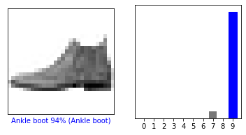
让我们看一看第0张图片的预测结果。正确预测标签为蓝色，错误预测，标签为红色。同时数字给出了标签预测正确的置信程度。(The number gives the percentage (out of 100) for the predicted label.)

i = 0
# 画布比例设置为 6:3
plt.figure(figsize=(6,3))
# 建立1行2列的子图，选中第一个子图
plt.subplot(1,2,1)
# 用函数plot_image绘制左图
plot_image(i, predictions[i], test_labels, test_images)
# 选中第二个子图
plt.subplot(1,2,2)
# 绘制右侧竖值条形图
plot_value_array(i, predictions[i],  test_labels)
# 显示图形
plt.show()

i = 12
plt.figure(figsize=(6,3))
plt.subplot(1,2,1)
plot_image(i, predictions[i], test_labels, test_images)
plt.subplot(1,2,2)
plot_value_array(i, predictions[i],  test_labels)
plt.show()

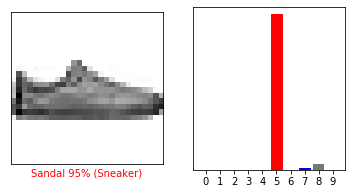
让我们多绘制一些带有预测的图像。但是请注意，尽管模型可能非常自信，但是仍可能预测错误。

# Plot the first X test images, their predicted labels, and the true labels.
# Color correct predictions in blue and incorrect predictions in red.
num_rows = 5 # 子图行数
num_cols = 3 # 子图列数
num_images = num_rows*num_cols # 子图总数
plt.figure(figsize=(2*2*num_cols, 2*num_rows)) # 设置宽高比

for i in range(num_images):
	# 选中当前子图
    plt.subplot(num_rows, 2*num_cols, 2*i+1)
    # 绘制左图
    plot_image(i, predictions[i], test_labels, test_images)
    # 选中当前子图
    plt.subplot(num_rows, 2*num_cols, 2*i+2)
    # 绘制右图
    plot_value_array(i, predictions[i], test_labels)
    
plt.tight_layout() # 调整子图的距离(不调整可能会重叠)
plt.show() # 图片显示

使用训练好的模型

最后，我们对单个图像进行预测。

# 从测试集中获取图像。
>>> img = test_images[1]
>>> print(img.shape)
(28, 28)

tf.keras模组对预测进行了优化，能够快速地对一批或者一组实例进行预测。据此，即使使用的是单个图像，也需要将其添加到列表中(就是维度加一)：

# 给图片添加一个维度以使其成为一个batch (Add the image to a batch where it's the only member.)

>>> img = (np.expand_dims(img,0))
>>> print(img.shape)
(1, 28, 28)

现在对图片做出预测：

>>> predictions_single = probability_model.predict(img)
>>> print(predictions_single)
>[[2.9944020e-05 3.4601690e-11 9.9824452e-01 7.7335160e-09 9.3144627e-04
  5.9004490e-10 7.9412595e-04 2.1851566e-13 3.1819016e-09 2.7337076e-15]]

plot_value_array(1, predictions_single[0], test_labels)
_ = plt.xticks(range(10), class_names, rotation=45)

keras.Model.predict返回一个包含列表的列表——即在一个batch中，所有的预测数组。(keras.Model.predict returns a list of lists—one list for each image in the batch of data.)
我们这样获取这一轮数据中唯一预测:

>>> np.argmax(predictions_single[0])
2

就像这样，模型预测了标签，就像我们期望的那样

---

以上便是tensorflow官方教程《Basic classification: Classify images of clothing》全部内容：
https://www.tensorflow.org/tutorials/keras/classification