计算机视觉——图像处理基础

1. PIL-Python图像库

PIL (Python Imaging Library)图像库提供了很多常用的图像处理及很多有用的图像基本操作。

Image.open(filename,mode)

返回一个Image对象，该对象有size,format,mode等属性，其中size表示图像的宽度和高度(像素表示);format表示图像的格式,常见的包括JPEG,PNG等格式;mode表示图像的模式，定义了像素类型还有图像深度等，常见的有RGB,HSV等。一般来说’L’(luminance)表示灰度图像,'RGB’表示真彩图像,'CMYK’表示预先压缩的图像。一旦你得到了打开的Image对象之后，就可以使用其众多的方法对图像进行处理了。

gray()

表示图像灰度化，在下面的代码中使用该函数使得原图像在显示的时候转换成灰度图像显示。

imshow()和pil_im.show()的区别

imshow()就可显示图片同时也显示其格式。
而pil_im.show()，结果仅显示图片，不显示格式。

convert(mode,matrix,dither,palette,colors)

convert方法可以改变图像的mode,一般是在’RGB’(真彩图)、‘L’(灰度图)、‘CMYK’(压缩图)之间转换。值得注意的是,从灰度图转换为真彩图，、实际上是很难恢复成原来的真彩模式的(不唯一)。
代码：

# -*- coding: utf-8 -*-
from PIL import Image
from pylab import *
# 添加中文字体支持
from matplotlib.font_manager import FontProperties
font = FontProperties(fname=r"c:\windows\fonts\SimSun.ttc", size=14)
figure()
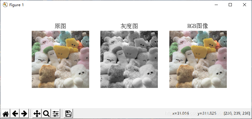
pil_im = Image.open('test.jpg')
gray() 
subplot(131)
title(u'原图',fontproperties=font)
axis('off')
imshow(pil_im)
pil_im = Image.open('test.jpg').convert('L')
subplot(132)
title(u'灰度图',fontproperties=font)
axis('off')
imshow(pil_im)
pil_im = Image.open('test.jpg').convert('RGB')
subplot(133)
title(u'RGB图像',fontproperties=font)
axis('off')
imshow(pil_im)
show()

运行结果：

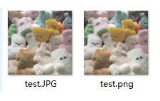
1.1 图片的格式转换

save(filename,format)

利用save()方法，PIL可以将图片保存问很多不同的图像格式。
注意，保存文件的文件名很重要，除非指定格式，否则这个库将会以文件名的扩展名作为格式保存。
代码：

from PIL import Image
from pylab import *
img = Image.open('test.JPG')
img.save('test.png', 'png')

运行结果：

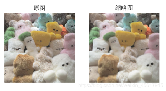
1.2 创建缩略图

thumbnail(size,resample)

该函数用于制作当前图片的缩略图, 参数size指定了图片的最大的宽度和高度，返回的是None。参数resample 是过滤器，只能是 NEAREST、BILINEAR、BICUBIC 或者 ANTIALIAS 之一。如果省略该变量，则默认为 NEAREST。

注意：在当前PIL的版本中，滤波器 BILINEAR 和 BICUBIC 不能很好地适应缩略图产生。用户应该使 用ANTIALIAS，图像质量最好。如果处理速度比图像质量更重要，可以选用其他滤波器。这个方法在原图上进行修改。

代码：

# -*- coding: utf-8 -*-
from PIL import Image
from pylab import *
# 添加中文字体支持
from matplotlib.font_manager import FontProperties
font = FontProperties(fname=r"c:\windows\fonts\SimSun.ttc", size=14)
figure()
# 缩略图
pil_im = Image.open('test.JPG')
subplot(121)
title(u'原图', fontproperties=font)
axis('off')
imshow(pil_im)
size = 128, 128
pil_im.thumbnail(size)
print(pil_im.size)
subplot(122)
title(u'缩略图', fontproperties=font)
axis('off')
imshow(pil_im)
pil_im.save('thumbnail.jpg') #保存缩略图
show()

运行结果：

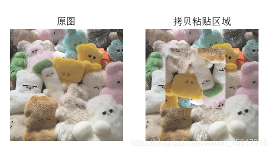
1.3拷贝并粘贴区域

crop(box)

该函数用于在图像上裁剪一个box矩形区域，box是一个有四个数字的元组(upper_left_x,upper_left_y,lower_right_x,lower_right_y),分别表示裁剪矩形区域的左上角x,y坐标,右下角的x,y坐标,规定图像的最左上角的坐标为原点(0,0),宽度的方向为x轴，高度的方向为y轴，每一个像素代表一个坐标单位。crop()返回的仍然是一个Image对象。

transpose(method)

该函数用于图像翻转或者旋转，method是transpose的参数，表示选择什么样的翻转或者旋转方式，可以选择的值有:
- Image.FLIP_LEFT_RIGHT,表示将图像左右翻转
- Image.FLIP_TOP_BOTTOM,表示将图像上下翻转
- Image.ROTATE_90,表示将图像逆时针旋转90°
- Image.ROTATE_180,表示将图像逆时针旋转180°
- Image.ROTATE_270,表示将图像逆时针旋转270°
- Image.TRANSPOSE,表示将图像进行转置(相当于顺时针旋转90°)
- Image.TRANSVERSE,表示将图像进行转置,再水平翻转

paste(region,box,mask)

该函数用于将一个图像粘贴到另一个图像，region是要粘贴的Image对象,box是要粘贴的位置，可以是一个两个元素的元组，表示粘贴区域的左上角坐标,也可以是一个四个元素的元组，表示左上角和右下角的坐标。如果是四个元素元组的话,box的size必须要和region的size保持一致，否则将会被convert成和region一样的size。

代码：

# -*- coding: utf-8 -*-
from PIL import Image
from pylab import *
# 添加中文字体支持
from matplotlib.font_manager import FontProperties
font = FontProperties(fname=r"c:\windows\fonts\SimSun.ttc", size=14)
figure()
# 缩略图
pil_im = Image.open('test.JPG')
subplot(121)
title(u'原图', fontproperties=font)
axis('off')
imshow(pil_im)
#拷贝粘贴区域
box = (100,100,400,400)
region = pil_im.crop(box)
region = region.transpose(Image.ROTATE_180)
pil_im.paste(region,box)
subplot(122)
title(u'拷贝粘贴区域', fontproperties=font)
axis('off')
imshow(pil_im)
show()

运行结果：

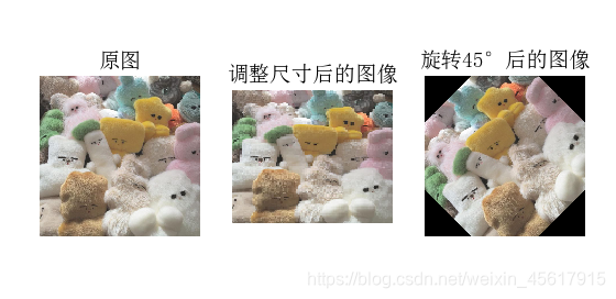
1.4 调整尺寸及旋转

resize(size,resample,box)

resize方法可以将原始的图像转换大小,size是转换之后的大小,resample是重新采样使用的方法，仍然有Image.BICUBIC，PIL.Image.LANCZOS，PIL.Image.BILINEAR，PIL.Image.NEAREST这四种采样方法，默认是PIL.Image.NEAREST,box是指定的要resize的图像区域，是一个用四个元组指定的区域(含义和上面所述box一致)。

rotate(angle,filter, expand)

该函数方法返回一个按照给定角度顺时钟围绕图像中心旋转后的图像拷贝。
变量filter应该是NEAREST、BILINEAR或者BICUBIC之一。如果省略该变量，或者图像模式为“1”或者“P”，则默认为NEAREST。
变量expand，如果为true，表示输出图像足够大，可以装载旋转后的图像。如果为false或者缺省，则输出图像与输入图像尺寸一样大。

代码：

# -*- coding: utf-8 -*-
from PIL import Image
from pylab import *
# 添加中文字体支持
from matplotlib.font_manager import FontProperties
font = FontProperties(fname=r"c:\windows\fonts\SimSun.ttc", size=14)
figure()
pil_im = Image.open('test.JPG')
subplot(131)
title(u'原图', fontproperties=font)
axis('off')
imshow(pil_im)
# 调整图像尺寸
pil_im = Image.open('test.JPG')
size = 120, 100
pil_im = pil_im.resize(size)
print (pil_im.size)
subplot(132)
title(u'调整尺寸后的图像', fontproperties=font)
axis('off')
imshow(pil_im)
# 旋转图像45°
pil_im = Image.open('test.JPG')
pil_im = pil_im.rotate(45)
subplot(133)
title(u'旋转45°后的图像', fontproperties=font)
axis('off')
imshow(pil_im)
show()

运行结果：

2. Matplotlib库

当在处理数学及绘图或在图像上描点、画直线、曲线时，Matplotlib是一个很好的绘图库，它比PIL库提供了更有力的特性。

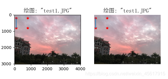
2.1 画图、描点和线

plot(x, y) # 默认为蓝色实线
plot(x, y, ‘r*’) # 红色星状标记
plot(x, y, ‘go-’) # 带有圆圈标记的绿线
plot(x, y, ‘ks:’) # 带有正方形标记的黑色点线

代码：

# -*- coding: utf-8 -*-
from PIL import Image
from pylab import *
# 添加中文字体支持
from matplotlib.font_manager import FontProperties
font = FontProperties(fname=r"c:\windows\fonts\SimSun.ttc", size=14)
im = array(Image.open('test1.JPG'))
figure()
# 画有坐标轴的
subplot(121)
imshow(im)
x = [100, 100, 800, 800]
y = [200, 800, 200, 800]
plot(x, y, 'r*')
plot(x[:2], y[:2])
title(u'绘图: "test.JPG"', fontproperties=font)
# 不显示坐标轴
subplot(122)
imshow(im)
x = [100, 100, 800, 800]
y = [200, 800, 200, 800]
plot(x, y, 'r*')
plot(x[:2], y[:2])
axis('off')  #显示坐标轴
title(u'绘图: "test.JPG.jpg"', fontproperties=font)
show()

运行结果：

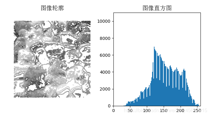
2.2 图像轮廓和直方图

n, bins, patches = plt.hist(arr, bins, normed, facecolor, alpha)

hist参数：
arr: 需要计算直方图的一维数组
bins: 直方图的柱数，可选项，默认为10
normed: 是否将得到的直方图向量归一化。默认为0
facecolor: 直方图颜色
alpha: 透明度
返回值 ：
n: 直方图向量，是否归一化由参数设定
bins: 返回各个bin的区间范围
patches: 返回每个bin里面包含的数据，是一个list
代码：

# -*- coding: utf-8 -*-
from PIL import Image
from pylab import *
# 添加中文字体支持
from matplotlib.font_manager import FontProperties
font = FontProperties(fname=r"c:\windows\fonts\SimSun.ttc", size=14)
im = array(Image.open('test.jpg').convert('L'))  # 打开图像，并转成灰度图像
figure()
subplot(121)
gray()
contour(im, origin='image')
axis('equal')
axis('off')
title(u'图像轮廓', fontproperties=font)
subplot(122)
hist(im.flatten(), 128)
title(u'图像直方图', fontproperties=font)
plt.xlim([0,260])
plt.ylim([0,11000])
show()

运行结果：

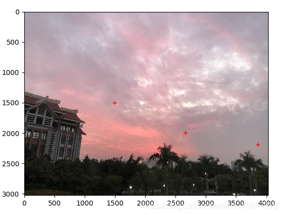
2.3交互注释

PyLab 库中的 ginput() 函数可以实现交互式标注。

在图像中点击，标记完毕输出标记点的位置。

代码：

from PIL import Image
from pylab import *

im = array(Image.open('test1.jpg'))
imshow(im)
print ('Please click 3 points')
imshow(im)
x = ginput(3)
print ('You clicked:', x)

show()

运行结果：

标注点的输出结果：

Please click 3 points
You clicked: [(1491.8636363636365, 1500.045454545454), 
(2661.8636363636365, 1990.9545454545453),
(3856.409090909092, 2187.3181818181815)]

3. NumPy库

3.1 图像数组表示

代码：

# -*- coding: utf-8 -*-
from PIL import Image
from pylab import *

im = array(Image.open('test.JPG'))
print (im.shape, im.dtype)
im = array(Image.open('test.JPG').convert('L'),'f')
print (im.shape, im.dtype)

运行结果：

(564, 564, 3) uint8
(564, 564) float32
[Finished in 0.8s]

3.2 灰度变换

代码：

 # -*- coding: utf-8 -*-
from PIL import Image
from numpy import *
from pylab import *

im = array(Image.open('test1.JPG').convert('L'))
print (int(im.min()), int(im.max()))

im2 = 255 - im  # invert image
print (int(im2.min()), int(im2.max()))

im3 = (100.0/255) * im + 100  # clamp to interval 100...200
print (int(im3.min()), int(im3.max()))

im4 = 255.0 * (im/255.0)**2  # squared
print (int(im4.min()), int(im4.max()))

figure()
gray()
subplot(1, 3, 1)
imshow(im2)
axis('off')
title(r'$f(x)=255-x$')

subplot(1, 3, 2)
imshow(im3)
axis('off')
title(r'$f(x)=\frac{100}{255}x+100$')

subplot(1, 3, 3)
imshow(im4)
axis('off')
title(r'$f(x)=255(\frac{x}{255})^2$')
show()

运行结果：

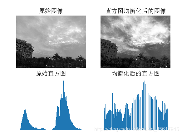
3.3 直方图均衡化

直方图均衡化是指将一幅图像的灰度直方图变平，使变换后的图像中每个灰度值的分布概率都相同。在对图像做进一步处理之前，直方图均衡化通常是对图像灰度值进行归一化的一个非常好 的方法，并且可以增强图像的对比度。

代码：

 # -*- coding: utf-8 -*-
from PIL import Image
from pylab import *
from PCV.tools import imtools

# 添加中文字体支持
from matplotlib.font_manager import FontProperties
font = FontProperties(fname=r"c:\windows\fonts\SimSun.ttc", size=14)

im = array(Image.open('test1.JPG').convert('L'))  # 打开图像，并转成灰度图像
#im = array(Image.open('../data/AquaTermi_lowcontrast.JPG').convert('L'))
im2, cdf = imtools.histeq(im)

figure()
subplot(2, 2, 1)
axis('off')
gray()
title(u'原始图像', fontproperties=font)
imshow(im)

subplot(2, 2, 2)
axis('off')
title(u'直方图均衡化后的图像', fontproperties=font)
imshow(im2)

subplot(2, 2, 3)
axis('off')
title(u'原始直方图', fontproperties=font)
#hist(im.flatten(), 128, cumulative=True, normed=True)
hist(im.flatten(), 128, normed=True)

subplot(2, 2, 4)
axis('off')
title(u'均衡化后的直方图', fontproperties=font)
#hist(im2.flatten(), 128, cumulative=True, normed=True)
hist(im2.flatten(), 128, normed=True)

show()

运行结果：

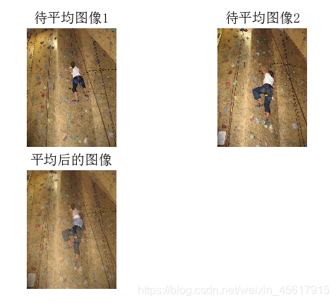
3.4 图像平均

图像平均操作是减少图像噪声的一种简单方式，通常用于艺术特效。

代码：

# -*- coding: utf-8 -*-
from PCV.tools.imtools import get_imlist
from PIL import Image
from pylab import *
from PCV.tools import imtools
# 添加中文字体支持
from matplotlib.font_manager import FontProperties
font = FontProperties(fname=r"c:\windows\fonts\SimSun.ttc", size=14)
filelist = get_imlist('data/avg/') #文件夹下的图片文件名(包括后缀名)
print (filelist)
avg = imtools.compute_average(filelist)
for impath in filelist:
        im1 = array(Image.open(impath))
        subplot(2, 2, filelist.index(impath)+1)
        imshow(im1)
        imNum=str(filelist.index(impath)+1)
        title(u'待平均图像'+imNum, fontproperties=font)
        axis('off')
subplot(2, 2, 3)
imshow(avg)
title(u'平均后的图像', fontproperties=font)
axis('off')
show()

运行结果：

4. SciPy模块

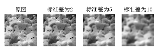
4.1 图像模糊

“模糊"的算法有很多种，其中有一种叫做"高斯模糊”（Gaussian Blur）。它将正态分布（又名"高斯分布"）用于图像处理。通常用它来减少图像噪声以及降低细节层次。 从数学的角度来看，图像的高斯模糊过程就是图像与正态分布做卷积。
代码：

 # -*- coding: utf-8 -*-
from PIL import Image
from pylab import *
from scipy.ndimage import filters

# 添加中文字体支持
from matplotlib.font_manager import FontProperties
font = FontProperties(fname=r"c:\windows\fonts\SimSun.ttc", size=14)

#im = array(Image.open('board.jpeg'))
im = array(Image.open('test.JPG').convert('L'))

figure()
gray()
axis('off')
subplot(1, 4, 1)
axis('off')
title(u'原图', fontproperties=font)
imshow(im)

for bi, blur in enumerate([2, 5, 10]):
  im2 = zeros(im.shape)
  im2 = filters.gaussian_filter(im, blur)
  im2 = np.uint8(im2)
  imNum=str(blur)
  subplot(1, 4, 2 + bi)
  axis('off')
  title(u'标准差为'+imNum, fontproperties=font)
  imshow(im2)

#如果是彩色图像，则分别对三个通道进行模糊
#for bi, blur in enumerate([2, 5, 10]):
#  im2 = zeros(im.shape)
#  for i in range(3):
#    im2[:, :, i] = filters.gaussian_filter(im[:, :, i], blur)
#  im2 = np.uint8(im2)
#  subplot(1, 4,  2 + bi)
#  axis('off')
#  imshow(im2)

show()

运行结果：

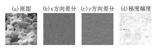
4.2 图像差分

4.2.1 图像差分

图像差分，就是把两幅图像的对应像素值相减，以削弱图像的相似部分，突出显示图像的变化部分。
代码：

# -*- coding: utf-8 -*-
from PIL import Image
from pylab import *
from scipy.ndimage import filters
import numpy

# 添加中文字体支持
from matplotlib.font_manager import FontProperties
font = FontProperties(fname=r"c:\windows\fonts\SimSun.ttc", size=14)

im = array(Image.open('test.jpg').convert('L'))
gray()

subplot(1, 4, 1)
axis('off')
title(u'(a)原图', fontproperties=font)
imshow(im)

# Sobel derivative filters
imx = zeros(im.shape)
filters.sobel(im, 1, imx)
subplot(1, 4, 2)
axis('off')
title(u'(b)x方向差分', fontproperties=font)
imshow(imx)

imy = zeros(im.shape)
filters.sobel(im, 0, imy)
subplot(1, 4, 3)
axis('off')
title(u'(c)y方向差分', fontproperties=font)
imshow(imy)

#mag = numpy.sqrt(imx**2 + imy**2)
mag = 255-numpy.sqrt(imx**2 + imy**2)
subplot(1, 4, 4)
title(u'(d)梯度幅度', fontproperties=font)
axis('off')
imshow(mag)

show()

运行结果：

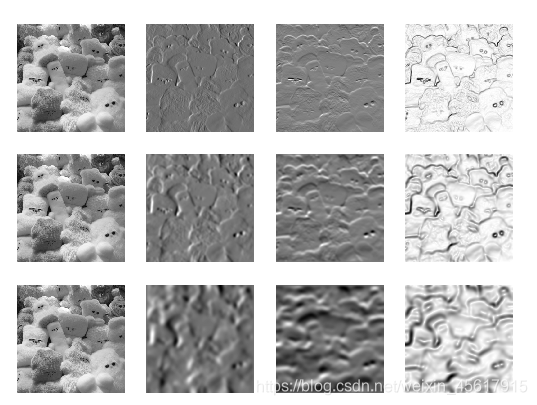
4.2.2 高斯差分

高斯差分与高斯拉普拉斯相似，都是先经过高斯平滑，再做差分，但这两个过程可结合成一起。

代码：

# -*- coding: utf-8 -*-
from PIL import Image
from pylab import *
from scipy.ndimage import filters
import numpy

# 添加中文字体支持
#from matplotlib.font_manager import FontProperties
#font = FontProperties(fname=r"c:\windows\fonts\SimSun.ttc", size=14)

def imx(im, sigma):
    imgx = zeros(im.shape)
    filters.gaussian_filter(im, sigma, (0, 1), imgx)
    return imgx


def imy(im, sigma):
    imgy = zeros(im.shape)
    filters.gaussian_filter(im, sigma, (1, 0), imgy)
    return imgy


def mag(im, sigma):
    # there's also gaussian_gradient_magnitude()
    #mag = numpy.sqrt(imgx**2 + imgy**2)
    imgmag = 255 - numpy.sqrt(imgx ** 2 + imgy ** 2)
    return imgmag


im = array(Image.open('test.jpg').convert('L'))
figure()
gray()

sigma = [2, 5, 10]

for i in  sigma:
    subplot(3, 4, 4*(sigma.index(i))+1)
    axis('off')
    imshow(im)
    imgx=imx(im, i)
    subplot(3, 4, 4*(sigma.index(i))+2)
    axis('off')
    imshow(imgx)
    imgy=imy(im, i)
    subplot(3, 4, 4*(sigma.index(i))+3)
    axis('off')
    imshow(imgy)
    imgmag=mag(im, i)
    subplot(3, 4, 4*(sigma.index(i))+4)
    axis('off')
    imshow(imgmag)

show()

运行结果：

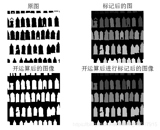
4.3 形态学-物体计数

思路：
1、通过形态学操作、阈值处理、距离变换等方法，使得各个轮廓分开
2、计算轮廓数量

代码：

# -*- coding: utf-8 -*-
from PIL import Image
from numpy import *
from scipy.ndimage import measurements, morphology
from pylab import *

"""   This is the morphology counting objects example in Section 1.4.  """

# 添加中文字体支持
from matplotlib.font_manager import FontProperties
font = FontProperties(fname=r"c:\windows\fonts\SimSun.ttc", size=14)

# load image and threshold to make sure it is binary
figure()
gray()
im = array(Image.open('houses.png').convert('L'))
subplot(221)
imshow(im)
axis('off')
title(u'原图', fontproperties=font)
im = (im < 128)

labels, nbr_objects = measurements.label(im)
print ("Number of objects:", nbr_objects)
subplot(222)
imshow(labels)
axis('off')
title(u'标记后的图', fontproperties=font)

# morphology - opening to separate objects better
im_open = morphology.binary_opening(im, ones((9, 5)), iterations=2)
subplot(223)
imshow(im_open)
axis('off')
title(u'开运算后的图像', fontproperties=font)

labels_open, nbr_objects_open = measurements.label(im_open)
print ("Number of objects:", nbr_objects_open)
subplot(224)
imshow(labels_open)
axis('off')
title(u'开运算后进行标记后的图像', fontproperties=font)

show()

运行结果：

Number of objects: 45
Number of objects: 48

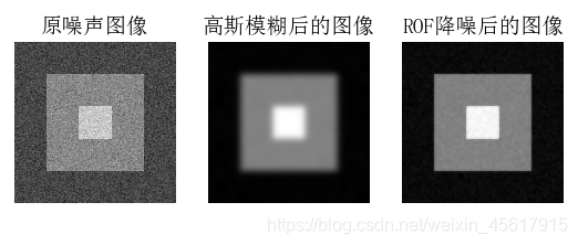
4.4 图像降噪

现实中的数字图像在数字化和传输过程中常受到成像设备与外部环境噪声干扰等影响，称为含噪图像或噪声图像。减少数字图像中噪声的过程称为图像降噪。

代码：

# -*- coding: utf-8 -*-
from pylab import *
from numpy import *
from numpy import random
from scipy.ndimage import filters
from scipy.misc import imsave
from PCV.tools import rof

""" This is the de-noising example using ROF in Section 1.5. """

# 添加中文字体支持
from matplotlib.font_manager import FontProperties
font = FontProperties(fname=r"c:\windows\fonts\SimSun.ttc", size=14)

# create synthetic image with noise
im = zeros((500,500))
im[100:400,100:400] = 128
im[200:300,200:300] = 255
im = im + 30*random.standard_normal((500,500))

U,T = rof.denoise(im,im)
G = filters.gaussian_filter(im,10)


# save the result
#imsave('synth_original.pdf',im)
#imsave('synth_rof.pdf',U)
#imsave('synth_gaussian.pdf',G)


# plot
figure()
gray()

subplot(1,3,1)
imshow(im)
#axis('equal')
axis('off')
title(u'原噪声图像', fontproperties=font)

subplot(1,3,2)
imshow(G)
#axis('equal')
axis('off')
title(u'高斯模糊后的图像', fontproperties=font)

subplot(1,3,3)
imshow(U)
#axis('equal')
axis('off')
title(u'ROF降噪后的图像', fontproperties=font)

show()

运行结果：