環境:window10 +のpython3
まず、NLTKをインストール
NLTK PIPのインストール
 #>ファイル- - >設定-またはPyCharm >プロジェクト通訳- > + 番号検索を- >パッケージをインストールします[matplotlibの、numpyの、パンダ一緒にインストールして、後で使用されます]
第二に、データNLTKブックをダウンロード
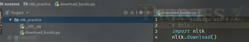
#download_books.py中

#- * -コーディング:UTF-8 - * -
#ノラ
輸入NLTKの
nltk.download()

特記事項:ダウンロードディレクトリ(ダウンロードディレクトリ)は、サンドボックス環境での共有ディレクトリとしてカタログをダウンロードするには、ここで、nltk_dataにする必要があり、自分の親ディレクトリを指定することができます。ディレクトリには、以下のいくつかのオファーを参照することができます見つけるために、ダウンロードディレクトリをカスタマイズする方法を知らなくても、検索ディレクトリに右である必要があります。
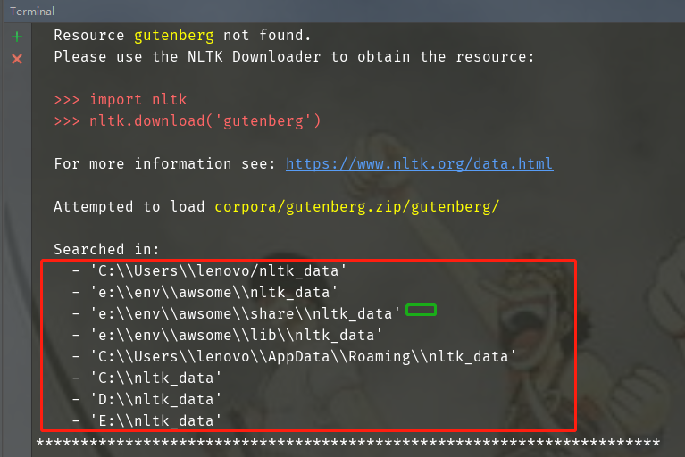
それは、ダウンロードに失敗した表示された場合は、すべてのパッケージを別途ダウンロード対応するライブラリNLTKダウンローダインターフェイスを見つけます。
データNLTKの本の第三に、使用
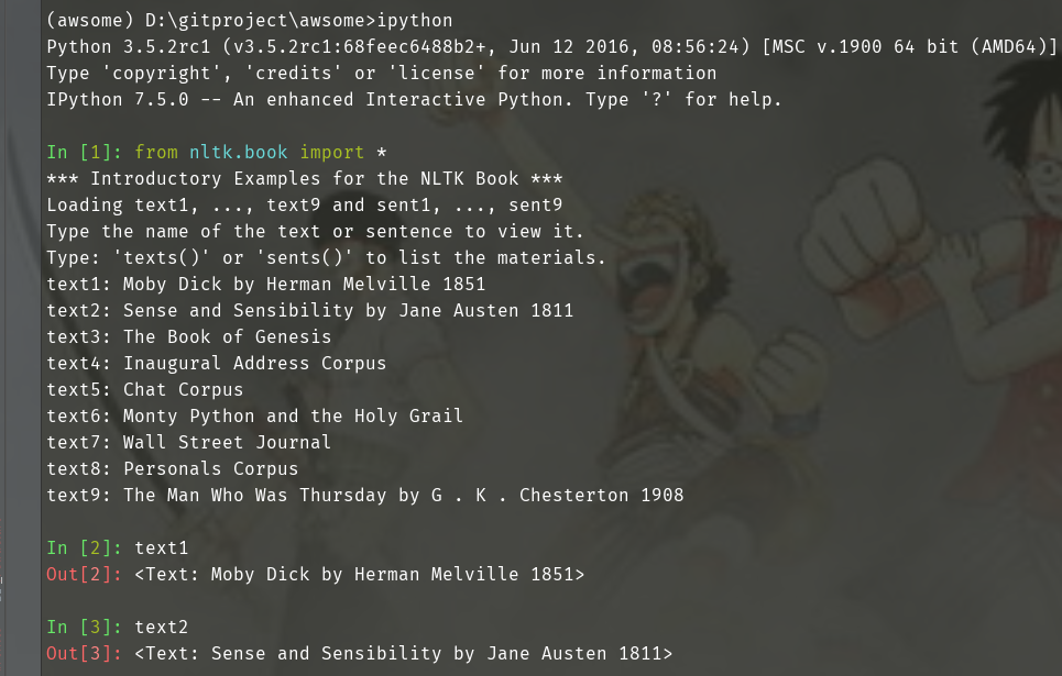
1.1本データセットを導入
#PyCharmオープンターミナル
#インストールIPython
PIP IPythonをインストール

から nltk.book インポート *

テキスト1

テキスト2
1.2 搜索文本
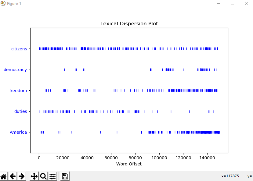
# concordance(word)函数 词汇索引word及上下文
text1.concordance("monstrous")
text2.concordance("affection")
text5.concordance("lol")

# similar(word)函数 搜索word相关词
text1.similar("monstrous")
text2.similar("monstrous")

# common_contexts([word1, word2])函数 搜索多个word共同上下文
text2.common_contexts(["monstrous", "very"])

# dispersion_plot([word1, word2, word3])函数 判断词在文本中的位置(每一竖线代表一个单词,从文本开始位置到指定词前面有多少给词) 离散图(使用matplotlib画图)
# generate() 生成随机文本
text3.generate()

1.3 词汇计数
# python语法
len(text3)
sorted(set(text3))
len(set(text3))
1.4 词频分布
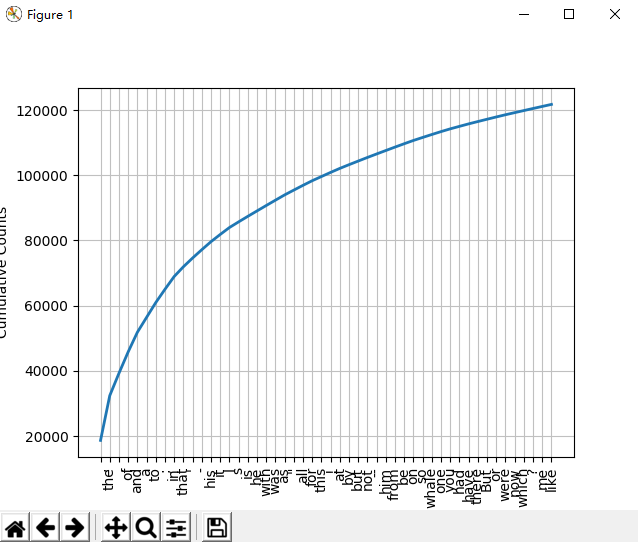
# FreqDist(text)函数 返回text文本中每个词出现的次数的元组列表
fdist1 = FreqDist(text1)

fdist1
FreqDist({',': 18713, 'the': 13721, '.': 6862, 'of': 6536, 'and': 6024, 'a': 4569, 'to': 4542, ';': 4072, 'in': 3916, 'that': 2982, ...})

print(fdist1)
<FreqDist with 19317 samples and 260819 outcomes>

# hapaxes()函数 返回低频词
len(fdist1.hapaxes())

# most_common(num)函数 返回高频词汇top50
fdist1.most_common(50)

fdist1.plot(50, cumulative=True) # top50词汇累计频率图
1.5 细粒度选择词
高频词和低频词提取出的信息量有限,研究文本中的长词提取出更多的信息量。采用集合论的一些符号:P性质,V词汇,w单个词符,P(w)当且仅当w词符长度大于15。表示为:{w | w ∈ V & P(w)}
V = set(text1)
long_words = [w for w in V if len(w) > 15]
len(long_words)

fdist5 = FreqDist(text5)
sorted(w for w in set(text5) if len(w) > 7 and fdist5[w] > 7)
1.6 词语搭配和双连词
# 词对称为双连词

# bigrams([word1, word2, word3]) 生成双连词 返回一个generator
list(bigrams(["a", "doctor", "with", "him"]))
Out[37]: [('a', 'doctor'), ('doctor', 'with'), ('with', 'him')]

# nltk中使用collocation_list()函数生成 很能体现文本风格
text4.collocation_list()
text8.collocation_list()
Out[44]:
['would like',
 'medium build',
 'social drinker',
 'quiet nights',
 'non smoker',
 'long term',
 'age open',
 'Would like',
 'easy going',
 'financially secure',
 'fun times',
 'similar interests',
 'Age open',
 'weekends away',
 'poss rship',
 'well presented',
 'never married',
 'single mum',
 'permanent relationship',
 'slim build']
1.7 计数词汇长度
# 统计text1文本词符长度和长度频次
[len(w) for w in text1]

fdist = FreqDist(len(w) for w in text1)

In [47]: fdist
Out[47]: FreqDist({3: 50223, 1: 47933, 4: 42345, 2: 38513, 5: 26597, 6: 17111, 7: 14399, 8: 9966, 9: 6428, 10: 3528, ...})

In [48]: fdist.most_common(10)
Out[48]:
[(3, 50223),
 (1, 47933),
 (4, 42345),
 (2, 38513),
 (5, 26597),
 (6, 17111),
 (7, 14399),
 (8, 9966),
 (9, 6428),
 (10, 3528)]

In [49]: fdist.max()
Out[49]: 3

In [50]: fdist[3]
Out[50]: 50223

In [51]: fdist.freq(3)
Out[51]: 0.19255882431878046

In [52]: fdist.freq(1)
Out[52]: 0.18377878912195814
1.8 函数说明
fdist.N()  # 样本总数

In [60]: fdist.freq(3)  # 给定样本的频率
Out[60]: 0.19255882431878046


In [55]: fdist.tabulate()  # 频率分布表
    3     1     4     2     5     6     7     8     9    10    11    12    13    14    15    16    17    18    20
50223 47933 42345 38513 26597 17111 14399  9966  6428  3528  1873  1053   567   177    70    22    12     1     1


fdist.plot()  # 频率分布图 (图1)
fdist.plot(cumulative=True)  # 累计频率分布图 (图2)
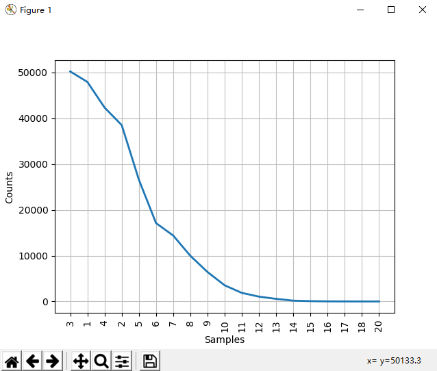
图1
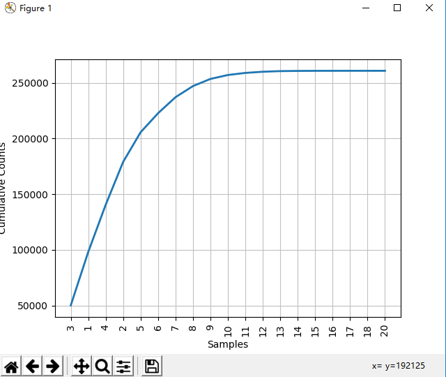
图2