Ensemble methods for unsupervised learning: clustering of similarity matrices

In machine learning, the term ensemble refers to combining multiple models in parallel. The idea is to use the wisdom of the crowd to form a better consensus on the final answer given.

This type of method has been widely studied and applied in the field of supervised learning, especially on classification problems with very successful algorithms like RandomForest. Some voting/weighting system is usually applied to combine the output of each individual model into a final, more robust and consistent output.

In the world of unsupervised learning, this task becomes even more difficult. First, because it encompasses the challenges of the field itself, we have no prior knowledge of the data to compare ourselves to any target. Second, because finding a suitable way to combine information from all models remains a problem, and there is no consensus on how to do this.

In this article, we discuss the best approach on this topic, namely clustering of similarity matrices.

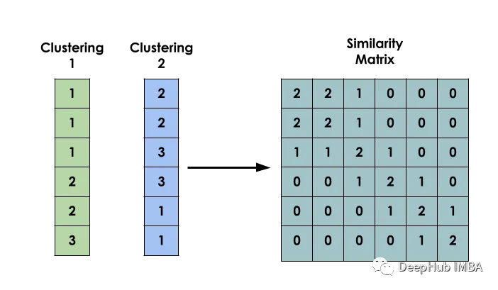
The main idea of this method is: given a data set X, create a matrix S such that Si represents the similarity between xi and xj. This matrix is constructed based on the clustering results of several different models.

binary co-occurrence matrix

The first step in building a model is to create a binary co-occurrence matrix between inputs.

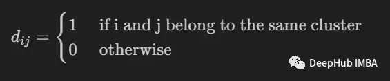
It is used to indicate whether two inputs i and j belong to the same cluster.

import numpy as np
 from scipy import sparse
 
 def build_binary_matrix( clabels ):
   
   data_len = len(clabels)
 
   matrix=np.zeros((data_len,data_len))
   for i in range(data_len):
     matrix[i,:] = clabels == clabels[i]
   return matrix
 
 labels = np.array( [1,1,1,2,3,3,2,4] )
 build_binary_matrix(labels)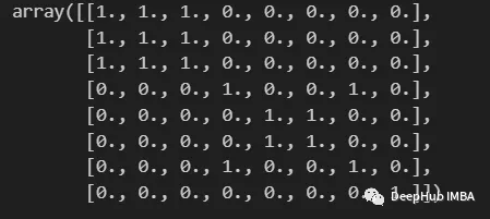

Construct similarity matrix using KMeans

We have constructed a function to binarize our clusters, and now we can enter the stage of constructing the similarity matrix.

We introduce here the most common method, which only involves calculating the average value between M co-occurrence matrices generated by M different models. defined as:

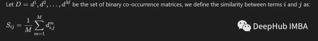
In this way, the similarity values of entries falling in the same cluster will be close to 1, while the similarity values of entries falling in different groups will be close to 0.

We will build a similarity matrix based on the labels created by the K-Means model. Conducted using the MNIST dataset. For simplicity and efficiency, we will only use 10,000 PCA-reduced images.

from sklearn.datasets import fetch_openml
 from sklearn.decomposition import PCA
 from sklearn.cluster import MiniBatchKMeans, KMeans
 from sklearn.model_selection import train_test_split
 
 mnist = fetch_openml('mnist_784')
 X = mnist.data
 y = mnist.target
 
 X, _, y, _ = train_test_split(X,y, train_size=10000, stratify=y, random_state=42 )
 
 pca = PCA(n_components=0.99)
 X_pca = pca.fit_transform(X)

To allow for diversity between models, each model is instantiated with a random number of clusters.

NUM_MODELS = 500
 MIN_N_CLUSTERS = 2
 MAX_N_CLUSTERS = 300
 
 np.random.seed(214)
 model_sizes = np.random.randint(MIN_N_CLUSTERS, MAX_N_CLUSTERS+1, size=NUM_MODELS)
 clt_models = [KMeans(n_clusters=i, n_init=4, random_state=214) 
               for i in model_sizes]
 
 for i, model in enumerate(clt_models):
   print( f"Fitting - {i+1}/{NUM_MODELS}" )
   model.fit(X_pca)

The following function is to create a similarity matrix

def build_similarity_matrix( models_labels ):
   n_runs, n_data = models_labels.shape[0], models_labels.shape[1]
 
   sim_matrix = np.zeros( (n_data, n_data) )
 
   for i in range(n_runs):
     sim_matrix += build_binary_matrix( models_labels[i,:] )
 
   sim_matrix = sim_matrix/n_runs
 
   return sim_matrix

Call this function:

models_labels = np.array([ model.labels_ for model in clt_models ])
 sim_matrix = build_similarity_matrix(models_labels)

The final result is as follows:

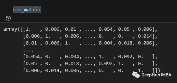
The information from the similarity matrix can still be post-processed before the final step, such as applying logarithmic, polynomial, etc. transformations.

In our case we will not make any changes.

Pos_sim_matrix = sim_matrix

Cluster similarity matrices

The similarity matrix is a way to represent the knowledge built by the collaboration of all clustering models.

Through it, we can intuitively see which entries are more likely to belong to the same cluster and which are not. But this information still needs to be converted into actual clusters.

This is done by using a clustering algorithm that can receive a similarity matrix as a parameter. Here we use SpectralClustering.

from sklearn.cluster import SpectralClustering
 spec_clt = SpectralClustering(n_clusters=10, affinity='precomputed',
                               n_init=5, random_state=214)
 final_labels = spec_clt.fit_predict(pos_sim_matrix)

Comparison with standard KMeans model

Let's compare it with KMeans to confirm whether our method is effective.

We will use NMI, ARI, cluster purity and class purity metrics to evaluate the standard KMeans model compared to our ensemble model. Additionally we will plot the contingency matrix to visualize which classes belong to each cluster.

from seaborn import heatmap
 import matplotlib.pyplot as plt
 
 def data_contingency_matrix(true_labels, pred_labels):
   
   fig, (ax) = plt.subplots(1, 1, figsize=(8,8))
 
   n_clusters = len(np.unique(pred_labels))
   n_classes = len(np.unique(true_labels))
   label_names =  np.unique(true_labels)
   label_names.sort()
 
   contingency_matrix = np.zeros( (n_classes, n_clusters) )
 
   for i, true_label in enumerate(label_names):
     for j in range(n_clusters):
       contingency_matrix[i, j] = np.sum(np.logical_and(pred_labels==j, true_labels==true_label))
 
   heatmap(contingency_matrix.astype(int), ax=ax,
           annot=True, annot_kws={"fontsize":14}, fmt='d')
   
   ax.set_xlabel("Clusters", fontsize=18)
   ax.set_xticks( [i+0.5 for i in range(n_clusters)] )
   ax.set_xticklabels([i for i in range(n_clusters)], fontsize=14)
   
   ax.set_ylabel("Original classes", fontsize=18)
   ax.set_yticks( [i+0.5 for i in range(n_classes)] )
   ax.set_yticklabels(label_names, fontsize=14, va="center")
   
   ax.set_title("Contingency Matrix\n", ha='center', fontsize=20)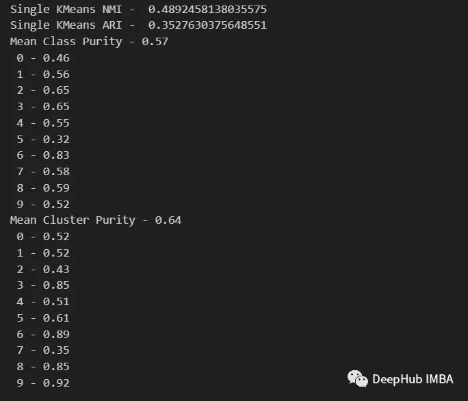

from sklearn.metrics import normalized_mutual_info_score, adjusted_rand_score
 
 def purity( true_labels, pred_labels ):
   
   n_clusters = len(np.unique(pred_labels))
   n_classes = len(np.unique(true_labels))
   label_names =  np.unique(true_labels)
 
   purity_vector = np.zeros( (n_classes) )
   contingency_matrix = np.zeros( (n_classes, n_clusters) )
 
   for i, true_label in enumerate(label_names):
     for j in range(n_clusters):
       contingency_matrix[i, j] = np.sum(np.logical_and(pred_labels==j, true_labels==true_label))
 
   purity_vector = np.max(contingency_matrix, axis=1)/np.sum(contingency_matrix, axis=1)
 
   print( f"Mean Class Purity - {np.mean(purity_vector):.2f}" ) 
   for i, true_label in enumerate(label_names):
     print( f" {true_label} - {purity_vector[i]:.2f}" ) 
 
   
   cluster_purity_vector = np.zeros( (n_clusters) )
   cluster_purity_vector = np.max(contingency_matrix, axis=0)/np.sum(contingency_matrix, axis=0)
 
   print( f"Mean Cluster Purity - {np.mean(cluster_purity_vector):.2f}" ) 
   for i in range(n_clusters):
     print( f" {i} - {cluster_purity_vector[i]:.2f}" ) 
 
 kmeans_model = KMeans(10, n_init=50, random_state=214)
 km_labels = kmeans_model.fit_predict(X_pca)
 
 data_contingency_matrix(y, km_labels)
 
 print( "Single KMeans NMI - ", normalized_mutual_info_score(y, km_labels) )
 print( "Single KMeans ARI - ", adjusted_rand_score(y, km_labels) )
 purity(y, km_labels)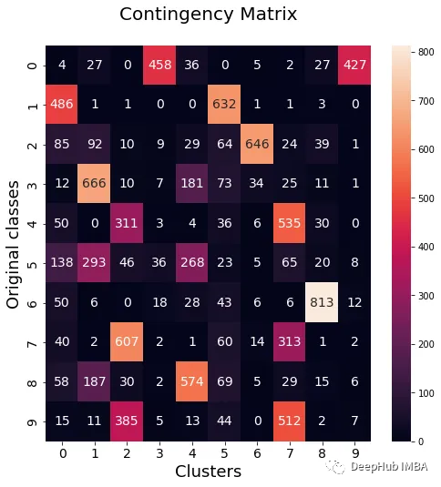

data_contingency_matrix(y, final_labels)
 
 print( "Ensamble NMI - ", normalized_mutual_info_score(y, final_labels) )
 print( "Ensamble ARI - ", adjusted_rand_score(y, final_labels) )
 purity(y, final_labels)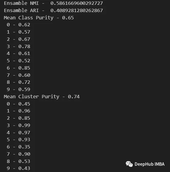

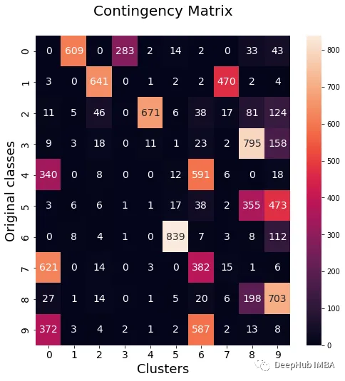
It can be seen from the above values that the Ensemble method can indeed improve the quality of clustering. We can also see more consistent behavior in the contingency matrix, with better distribution classes and less "noise".

Cited in this article

Strehl, Alexander, and Joydeep Ghosh. “Cluster ensembles — -a knowledge reuse framework for combining multiple partitions.” Journal of machine learning research 3.Dec (2002): 583–617.

Fred, Ana, and Anil K. Jain. “Combining multiple clusterings using evidence accumulation.” IEEE transactions on pattern analysis and machine intelligence 27.6 (2005): 835–850.

Topchy, Alexander, et al. “Combining multiple weak clusterings.” Third IEEE International Conference on Data Mining. IEEE, 2003.

Fern, Xiaoli Zhang, and Carla E. Brodley. “Solving cluster ensemble problems by bipartite graph partitioning.” Proceedings of the twenty-first international conference on Machine learning. 2004.

Gionis, Aristides, Heikki Mannila, and Panayiotis Tsaparas. “Clustering aggregation.” ACM Transactions on Knowledge Discovery from Data (TKDD) 1.1 (2007): 1–30.

作者：Nielsen Castelo Damasceno Dantas / DEEPHUB