Accurate analysis of multiple linear regression regress function in matlab (with example code)
Table of contents
Second, the parameters in the regress function
foreword
The regress function is very powerful. It can be used for multiple linear regression analysis. It can not only obtain the coefficients in the linear regression function, but also return a series of meaningful statistical parameters, which is helpful for our analysis of the regression function. This time introduces the basic functions of the regress function and then configures it to show how to use the regress function with specific examples.
Tip: The following is the text of this article, all of which are original by the author himself. It is not easy to write an article. I hope you will attach a link to this article when reposting.
1. What is regress?
The regress function is used for multiple linear regression (Multiple linear regression). To put it simply, for example, given several sets of data about y, x1, and x2, they satisfy a certain relationship. For example, we can use this function to find the values of a, b, c, and d with the help of known data. .
Second, the parameters in the regress function
The usage format of the regress function is as follows:
[b,bint,r,rint,stats] = regress(y,X,alpha);b ------ returns a vector b of coefficient estimates for a multiple linear regression of the responses in vector y on the predictors in matrix x . The matrix x must include a column of ones. b is a column vector returned is The coefficient estimation vector b of the multiple linear regression obtained under the data of x and y , the matrix x must contain a column of 1. As for why x needs to contain a column of 1, see the analysis of x below .
bint ------ returns a matrix bint of 95% confidence intervals for the coefficient estimates. Returns a matrix bint of 95% confidence intervals for the coefficient estimates. bint is a matrix with multiple rows and two columns that returns the 95% confidence intervals for the coefficient estimates. To put it simply, the understanding of confidence interval is reliability. After learning probability theory, you will understand what confidence interval is. Each line of bint has two values, which can be regarded as the upper and lower bounds of an interval. The interval of each line of it is the 95% confidence interval of the parameter in each line of parameter b .
r ------returns an additional vector r of residuals. r is short for residual, which means residual. r returns a column vector, and each value in r is obtained by subtracting the predicted y value from the real data y, called the residual.
rint ------returns a matrix rint of intervals that can be used to diagnose outliers. What is returned is also a matrix with multiple rows and two columns. Its understanding can be the same as that of bint , except that the credible interval of r is judged at this time .
stats ------returns a vector stats that contains the statistic, the F -statistic and its p -value, and an estimate of the error variance. The translation of stats into Chinese means 'statistics', and what is returned is a vector containing A row vector of various statistics, including
a row vector of the statistic, the observed F statistic, and the p-value and error variance estimate of the test.
The closer to 1, the more significant the regression equation is;
when it is rejected
, the larger F is, the more significant the regression equation is;
when it is rejected
. This also involves the knowledge of hypothesis testing of probability theory, which will be understood after studying probability theory. Here we can only focus on
the value of the correlation coefficient, which can help us judge the pros and cons of the regression equation.
y ------ is a column vector, which is known data.
x ------ is a matrix, its first column is all 1, whether there is a column that is all 1 determines whether the regression equation contains a constant parameter for fitting, that is, whether the parameter d in is fitted Come out. The column corresponding to all 1s in the program is generally expressed as: ones(size(y)), where x1 and x2 are independent variables in the multiple linear regression equation and are known data. as follows:
x=[ones(size(y)),x1,x2];alpha------significant level, the default is 0.05.
3. Example analysis
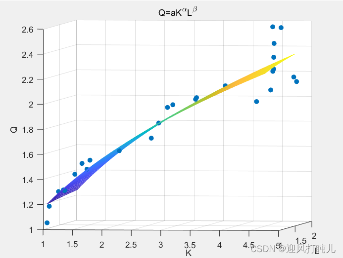
Here we fit an equation , Q, K, and L are known data, K, L are regarded as independent variables, and Q is regarded as a dependent variable, and the values of a and sum need to be
obtained
. Obviously it is not a linear equation, then we take the logarithm on both sides of it at the same time, and get:
, at this time, LnQ is regarded as a whole, as the dependent variable, LnK and LnL are regarded as two wholes, as independent variables, then become into a linear equation.
The program used in the example is as follows:
Q=[1.05 1.18 1.29 1.30 1.30 1.42 1.50 1.52 1.46 1.60 1.69 1.81 1.93 1.95 2.01 2.00 2.09 1.96 2.20 2.12 2.16 2.08 2.24 2.56 2.34 2.45 2.58]';
y=log(Q);
K=[1.04 1.06 1.16 1.22 1.27 1.37 1.44 1.53 1.57 2.05 2.51 2.63 2.74 2.82 3.24 3.24 3.61 4.10 4.36 4.77 4.75 4.54 4.54 4.58 4.58 4.58 4.54]';
x1=log(K);
L=[1.05 1.08 1.18 1.22 1.17 1.30 1.39 1.47 1.31 1.43 1.58 1.59 1.66 1.68 1.65 1.62 1.86 1.93 1.96 1.95 1.90 1.58 1.67 1.82 1.60 1.61 1.64]';
x2=log(L);
x=[ones(size(y)),x1,x2];
[b,bint,r,rint,stats] = regress(y,x);
a=exp(b(1));alpha=b(2);beta=b(3);
R=stats(1);
% % %Plot the data and the model.% % %
scatter3(x1,x2,y,'filled'); %scatter3函数用于画三维散点图
hold on;
x1fit = min(x1):0.05:max(x1);
x2fit = min(x2):0.05:max(x2);
[X1FIT,X2FIT] = meshgrid(x1fit,x2fit);%meshgrid用于画曲面图
YFIT = b(1) + b(2)*X1FIT + b(3)*X2FIT ;
mesh(X1FIT,X2FIT,YFIT);
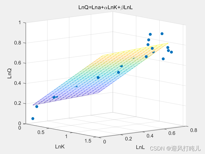
title("LnQ=Lna+\alphaLnK+\betaLnL");
xlabel('LnK');
ylabel('LnL');
zlabel('LnQ');
view(50,10);
hold off;
% % %Plot the data and the model.% % %
figure(2);
x1=exp(x1);
x2=exp(x2);
y=exp(y);
scatter3(x1,x2,y,'filled');
hold on;
x1fit = min(x1):0.05:max(x1);
x2fit = min(x2):0.05:max(x2);
[X1FIT,X2FIT] = meshgrid(x1fit,x2fit);
YFIT = a*(X1FIT.^alpha).*(X2FIT.^beta);
mesh(X1FIT,X2FIT,YFIT);
title("Q=aK^{\alpha}L^{\beta}");
xlabel('K');
ylabel('L');
zlabel('Q');
view(50,20);%view函数用于调整我们看三维图形的视角
hold off;
After running the program, the regress function will return to us the values of various parameters. For example vector b :
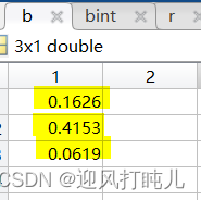
These three values are the values of Lna, and , respectively
.
Another example is the matrix bint:

The two numbers in each row are the confidence intervals of the previous b vectors, that is, the 95% confidence intervals of Lna, and in the above three rows.
Another example is the column vector r :
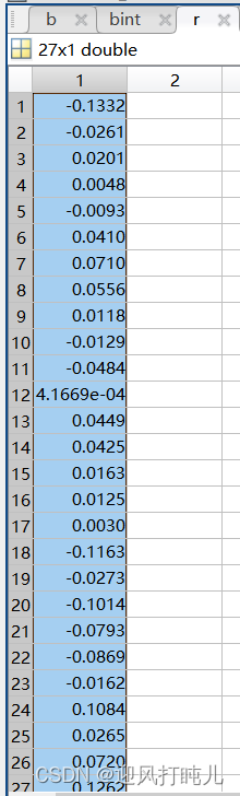
The value of each row is equal to the real data LnQ minus the fitted data LnQ, which is called the residual.
Another example is matrix rint:
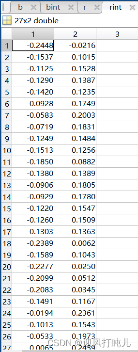
The two numbers in each row are regarded as an interval, which is understood as the credible interval of the corresponding residual.
Another example is the row vector stats:

Just focus on the value, the closer to 1 the better.
After running the program, two graphs will be obtained to help us intuitively feel the fitting effect. The two graphs are essentially the same. The difference is that one takes the logarithm and the other does not take the logarithm. For details, see the figure below title.
The above examples only fit the primary term of the independent variable, so how to write it in the program if it contains the quadratic term, for example, only need to modify X, please refer to the following for details:
x=[ones(size(y)),x1.^2,x2.^2,x1.*x2,x1,x2];
[b,bint,r,rint,stats] = regress(y,x);
Summarize
The above is the content to be shared this time. This article introduces the use of the regress function in detail. Once you learn it, let’s do it quickly.