Table of contents
In fact, I have come into contact with the robot toolbox in class before, and have done experiments step by step with the teacher's courseware, but I have never used it after the course. . .
Now, due to the future topic, and the MBD course required by the teacher, I will use it, so let's study it carefully.
❤ 2020.5.9 ❤
After studying for so many years, I haven't studied matlab much, and I feel like I'm losing money. But what should come will always come. The graduation project and MBD made me have to study matlab seriously. Although the basic operations are a little bit sloppy now, various toolboxes are the essence of matlab.
The most concise zero-based tutorial for matlab: Matlab Introductory Tutorial [Basic Direction]
Of course, what is said here is really too basic, so that people who have learned any programming language will find it simple. Of course, it is still possible to understand the basic grammar format of matlab.
Download, install and basic knowledge
Download and install Robot Toolbox
matlab's robot toolbox is a third-party toolbox. I tried to download it directly in the additional function explorer of matlab. I can only download it from the author's official website.
The author's name is Peter Corke, and his personal website and the official website of Robot Toolbox are:
Peter Corke
The author also wrote a book for the toolbox, which can be regarded as the manual of the toolbox. You can download the English version directly on the website, and there is also an official Chinese version, but there is no download on the official website. Of course, there are other magical methods besides buying. available. . .
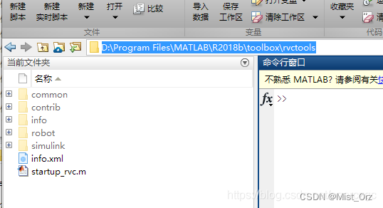
After downloading the toolkit from the author's personal website or the official website of the robot toolbox, unzip and copy it to the toolbox folder of matlab Copy the
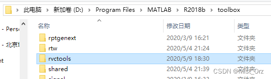
path to the main window of matlab, press Enter to enter,
double-click to open startup_rvc.m, and click to run
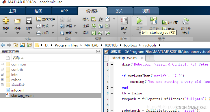
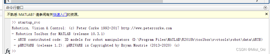
the command The window prompts as follows, the installation is successful.
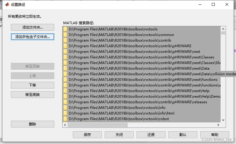
Then add the path
and enter ver in the command window to check whether the robot toolbox is installed successfully
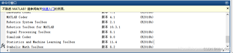
, which means it is successful.
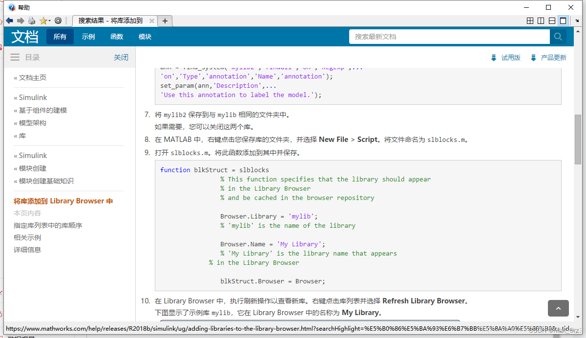
Another step is not necessary, but it is mentioned in the file of MBD course, that is to add the function block of the robot toolbox to the library browser of simulink. First, create a script file slblocks under MATLAB\R2018b\toolbox\rvctools\simulink. m, then add the following
function blkStruct = slblocks
%SLBLOCKS Defines a block library.
% Library's name. The name appears in the Library Browser's
% contents pane.
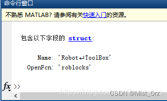
blkStruct.Name = ['Robot' sprintf('\n') 'ToolBox'];
% The function that will be called when the user double-clicks on
% the library's name. ;
blkStruct.OpenFcn = 'roblocks';
% The argument to be set as the Mask Display for the subsystem. You
% may comment this line out if no specific mask is desired.
% Example: blkStruct.MaskDisplay = 'plot([0:2*pi],sin([0:2*pi]));';
% No display for now.
% blkStruct.MaskDisplay = '';
% End of blocks
Run, the following content should be displayed successfully.
The function of this file can refer to the help file of matlab, "Add the library to the Library Browser" field, but the content of this script is still very different from the help file. After all, this script is The robot toolbox provided in the software package provided by the mbd course can be used anyway. Well
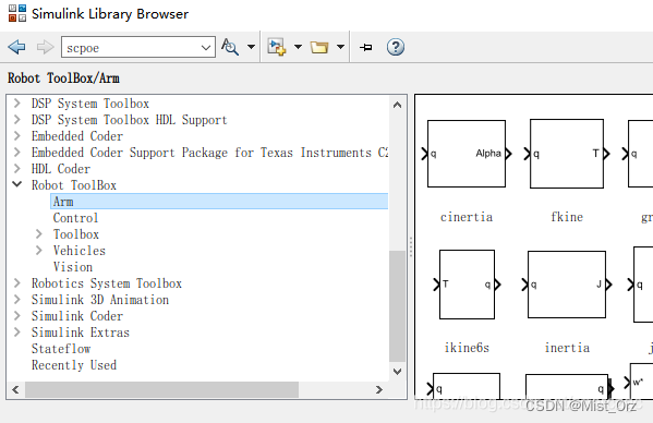
, start simulink, and then you can find the contents of the robot toolbox in the library browser
. In addition to downloading the installation package, you can also download RTB from the official website .mltbx file, and then open it directly or open it in matlab to install the toolbox, but I don’t know how to call the simulink function block after installation.
❤ 2020.5.10 ❤
Below is a record of how to use the basic functions of the robot toolbox. For the source of content, see
→→→ Liu Haitao LHT
This is the first episode of the series, I won't post the rest
How to use basic functions
Pose description
〇The two-dimensional space pose describes
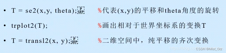
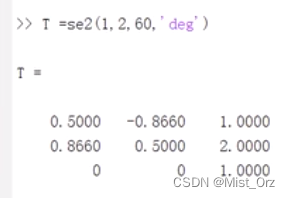
the rotation angle of the SE2() function using the angle system, such as data such as pi/3. Note that SE should be capitalized (at least my lowercase is not acceptable), and when the angle system data needs to be used, it should be written in the format of T=SE2(1,2,60,'deg').

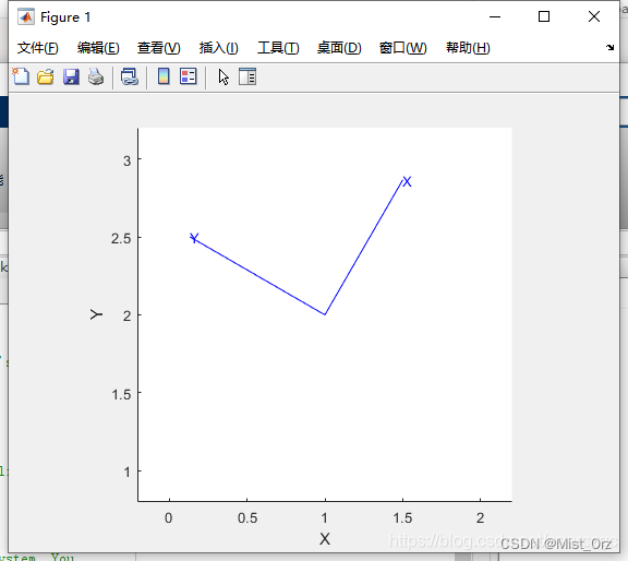
The parameter of the trplot2() function is the rotation matrix generated by the SE2() function, and the rotated coordinates are generated.
※ If it needs to be expressed in angle system, it should be written like this
〇Three-dimensional space pose description
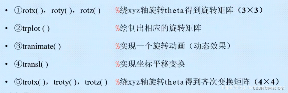
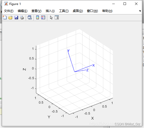
rotx/roty/rotz is to rotate the specified angle around the axis to generate a three-dimensional transformation matrix. If you use the angle system, you must add 'deg'.
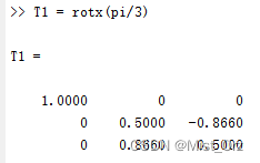
trplot is a drawing command for three-dimensional space.
Tranimate() is to display the transformation action with animation.
transl() is three-dimensional space translation.
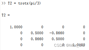
trotx/torty/trotz is a three-dimensional homogeneous transformation matrix, and the output is a 4x4 matrix, except that there is a 1 in the matrix besides the 3x3 matrix representing the rotation angle.
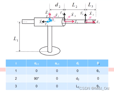
Build a robot model
〇Link class
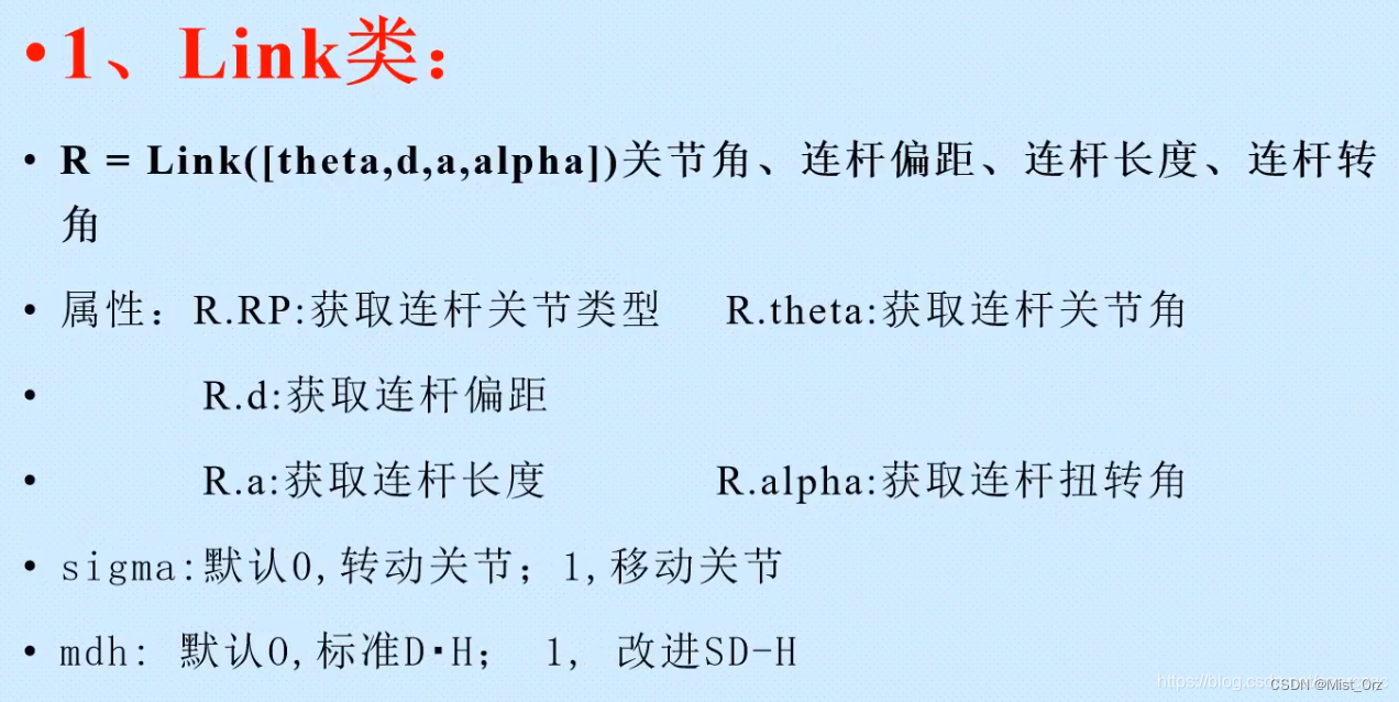
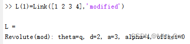
The function of Link() function is to establish the DH parameters of the robot in matlab. First, it is necessary to model the DH parameters of the robot. Of course, this is the content of robotics. I will write a detailed introduction to robotics when I have a chance. study notes.
The effect of the link function of a single joint is as follows. Note that 'modified' must be added when using the improved DH method, otherwise the standard DH is used by default.
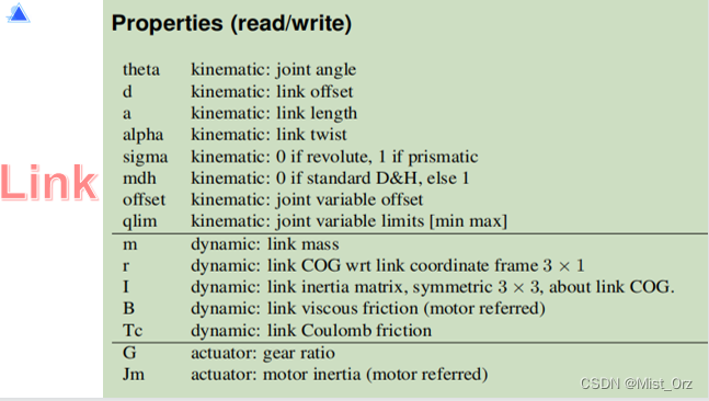
After the link is established, you can query the properties of the link, such as querying the joint type.
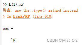
See the picture for the properties that can be queried. I don’t know what sigma is for, it’s not mentioned in the tutorial
〇SerialLink class
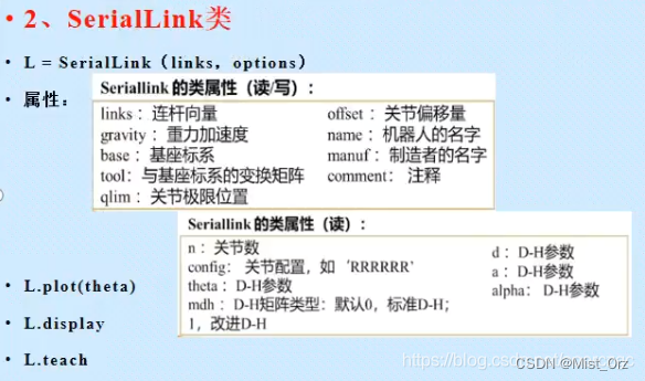
is used to integrate the defined links into a robot.
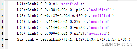
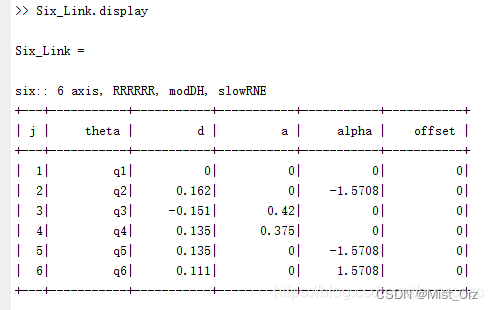
For example, to run such a script, first define 6 links, then integrate the links
and then query the properties of Six_Link through commands, for example,
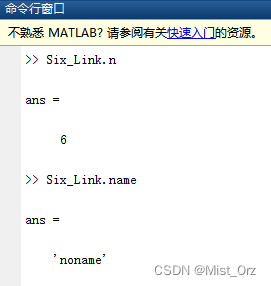
the type of properties can be queried from the above figure.
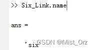
Attributes can be modified after definition, or added during definition, such as

Then query
about .plot(theta), this is an important drawing command, which displays the position of the robot by specifying the angle of each joint angle, such as
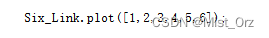
Images can be obtained
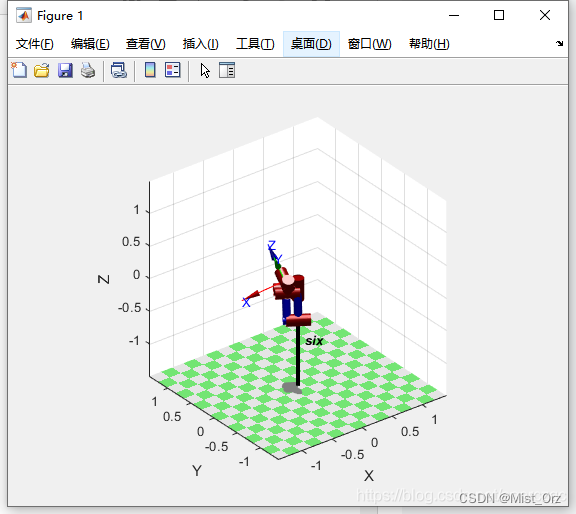
Don't mind these distorted joints.
Regarding .display, it is to display all the parameters of the robot.
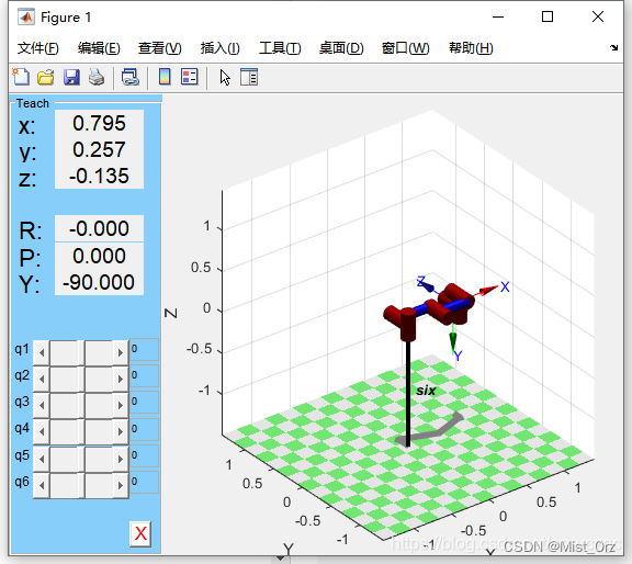
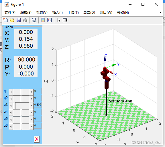
About .teach, it is teaching mode, graphic teaching device, input
After that, such a thing will be displayed, in which you can change the angle of each joint.
Robot Kinematics
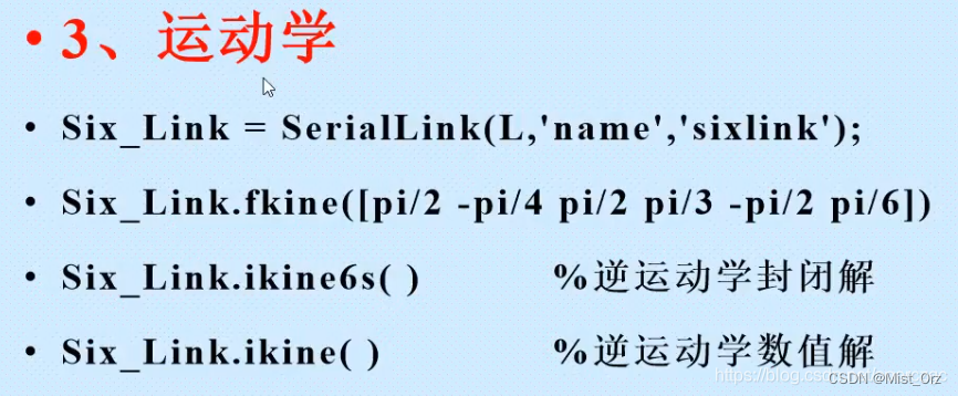
Forward kinematics
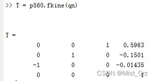
The .fkine() command is a kinematics positive solution, which generates the end-to-end transformation matrix corresponding to the joint angle, such as

inverse kinematics
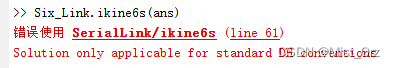
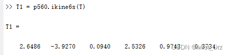
Regarding .ikine6s() and yu.ikine(), these two are inverse solutions for kinematics, and 6s is a closed solution. This command can only be applied to the model established by the standard DH modeling method. If it is improved DH will report an error, I don't know why. . .
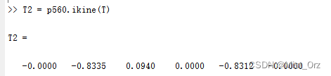
Then use .ikine(), but. . .
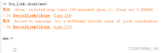
It should be a problem of model building, but the video says that this function is problematic. If you want to realize the inverse calculation, you need to write the function yourself. . . I go. . .
Let's go ahead.
☆ One like break
Take the puma560 model built in matlab as an example
First open puma560
As shown in the figure, some parameters and instructions of puma560
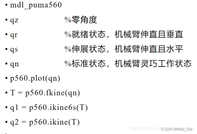
can be drawn with drawing instructions, such as
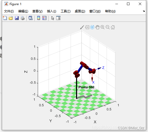
Kinematics positive solution
Kinematics anti-solution Closed solution
Kinematics anti-solution Numerical solution
Shocked, it is different. . .
Analysis on Forward Kinematics
According to the paper "Research on Zero-force Control and Collision Detection Technology of Collaborative Robots"_Chen Saixuan
〇According to the expression, judge whether the established DH model is a standard type (Standard DH) or a modified type (Modified DH). The
first element of the third and fourth lines is 0 is the standard type, and the one that
grows like this is the improved
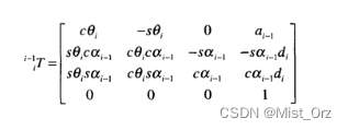
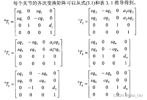
type〇The robot reverses the script program Write
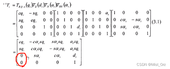
1. Express the derived transformation matrix in the script file
syms a2 a3 d1 d4 d5 d6 theta1 theta2 theta3 theta4 theta5 theta6
T01 = [ cos(theta1) 0   sin(theta1)     0;
        sin(theta1) 0   -cos(theta1)    0;
        0           1   0               d1;
        0           0   0               1];

T12 =[  cos(theta2) -sin(theta2)    0   a2*cos(theta2);
        sin(theta2) cos(theta2)     0   a2*sin(theta2);
        0           0               1   0;
        0           0               0   1];

T23 =[  cos(theta3) -sin(theta3)    0   a3*cos(theta3);
        sin(theta3) cos(theta3)     0   a3*sin(theta3);
        0           0               1   0;
        0           0               0   1];

T34 = [ cos(theta4) 0               sin(theta4)     0;
        sin(theta4) 0               -cos(theta4)    0;
        0           1               0               d4;
        0           0               0               1];

T45=[   cos(theta5) 0               -sin(theta5)    0;
        sin(theta5) 0               cos(theta5)     0;
        0           -1              0               d5;
        0           0               0               1];
T56=[   cos(theta6) -sin(theta6)    0               0;
        sin(theta6) cos(theta6)     0               0;
        0           0               1               d6;
        0           0               0               1];
T=T01*T12*T23*T34*T45*T56
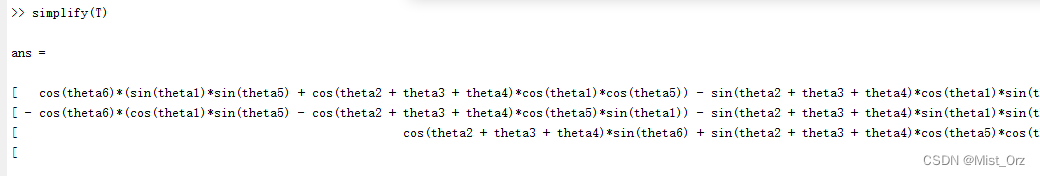
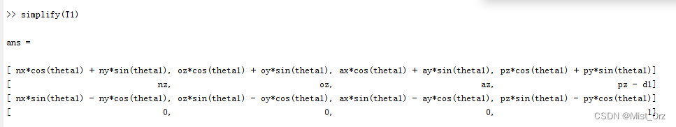
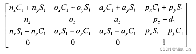
2. Simplify the matrix
with the simplify() function
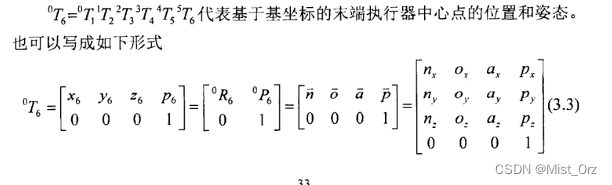
Analysis on Inverse Kinematics
Construct 4x4 equations by left multiplying the inverse of T01

syms a2 a3 d1 d4 d5 d6 theta1 theta2 theta3 theta4 theta5 theta6 nx ny nz ox oy oz ax ay az px py pz
T01 = [ cos(theta1) 0   sin(theta1)     0;
        sin(theta1) 0   -cos(theta1)    0;
        0           1   0               d1;
        0           0   0               1];

T12 =[  cos(theta2) -sin(theta2)    0   a2*cos(theta2);
        sin(theta2) cos(theta2)     0   a2*sin(theta2);
        0           0               1   0;
        0           0               0   1];

T23 =[  cos(theta3) -sin(theta3)    0   a3*cos(theta3);
        sin(theta3) cos(theta3)     0   a3*sin(theta3);
        0           0               1   0;
        0           0               0   1];

T34 = [ cos(theta4) 0               sin(theta4)     0;
        sin(theta4) 0               -cos(theta4)    0;
        0           1               0               d4;
        0           0               0               1];

T45=[   cos(theta5) 0               -sin(theta5)    0;
        sin(theta5) 0               cos(theta5)     0;
        0           -1              0               d5;
        0           0               0               1];
T56=[   cos(theta6) -sin(theta6)    0               0;
        sin(theta6) cos(theta6)     0               0;
        0           0               1               d6;
        0           0               0               1];

TT=[    nx oz ax pz;
        ny oy ay py;
        nz oz az pz;
        0  0  0  1];
T1=inv(T01)*TT
T2=T01*T12*T23*T34*T45*T56
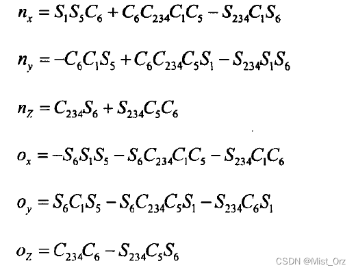
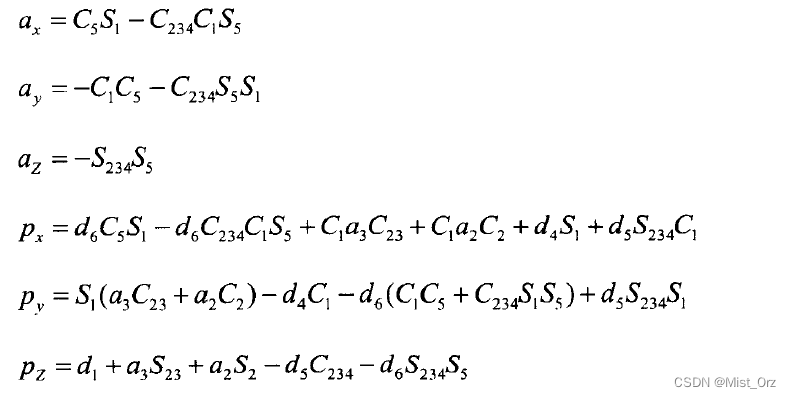
Simplify T1, T2
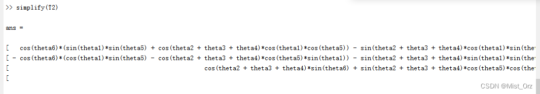
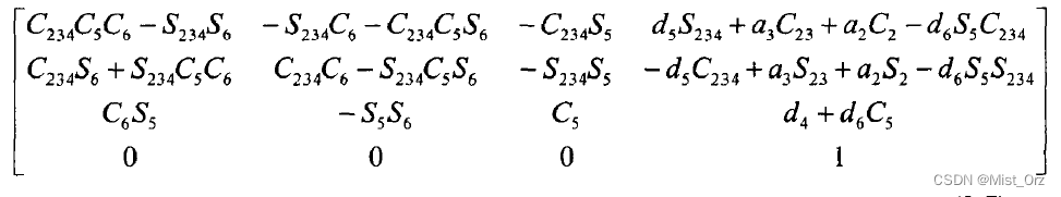
(The following is the original text of the paper)
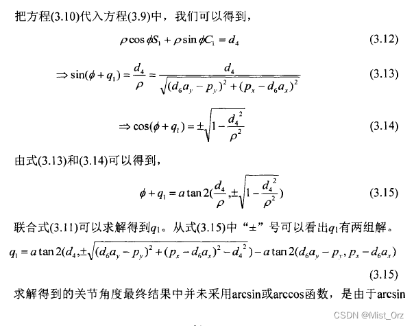
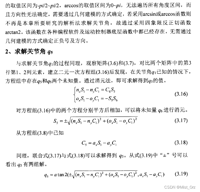
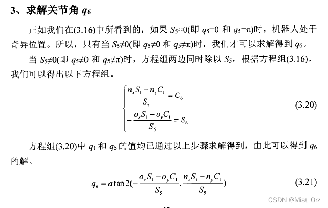
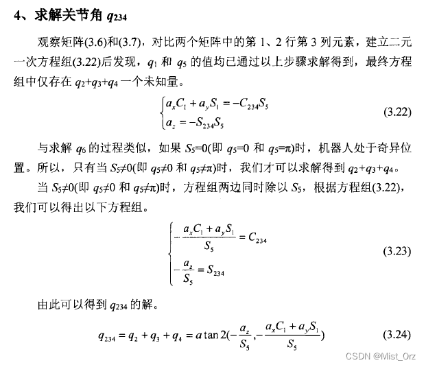
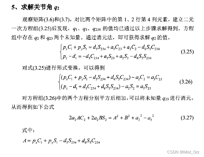
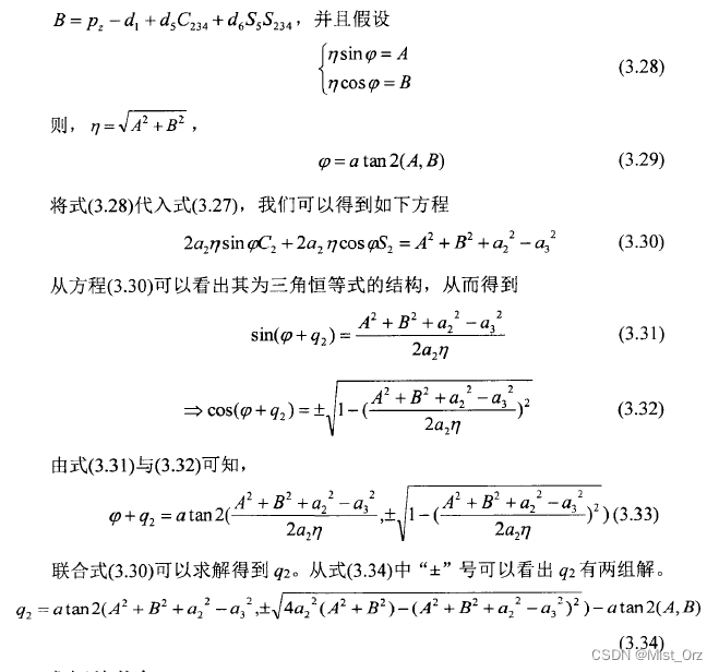
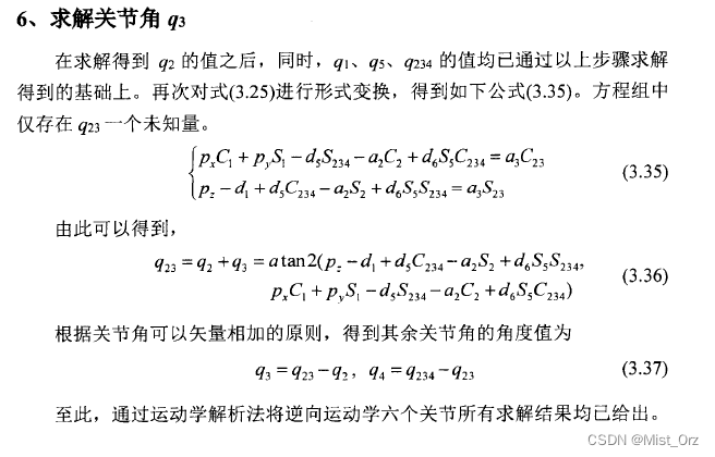
Solve the joint angle
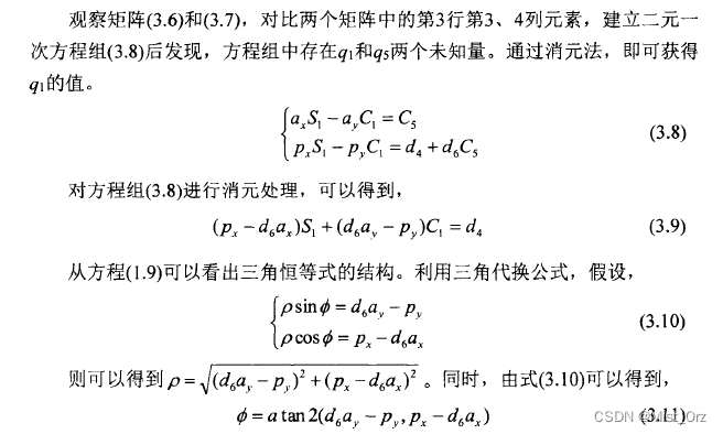
. Note that atan2() is a very important function. This must be used to solve the problem here. I don’t understand what the teacher said.
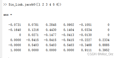
Jacobian matrix
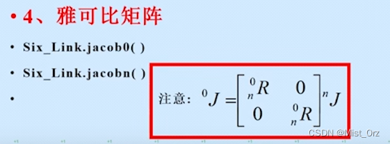
First build the robot model and then
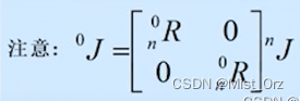
.jacob0(): for the base coordinates
. jacobn(): for the tool coordinates.
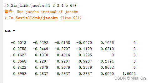
The two can be transformed
❤ 2022.6.8 ❤
robot with moving joints
Models that come with Robot Toolbox

An animation of the robot can be viewed
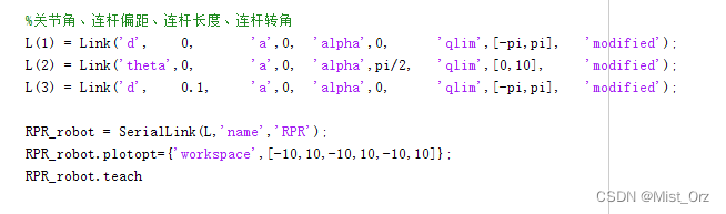
Build your own mobile joint robot model
※ Note: In the process of building a model, don’t write whoever is a variable in “d” and “theta” in the Link() function.
%关节角、连杆偏距、连杆长度、连杆转角
L(1) = Link('d',    0,       'a',0,  'alpha',0,      'qlim',[-pi,pi],	'modified');
L(2) = Link('theta',0,       'a',0,  'alpha',pi/2,   'qlim',[0,10],     'modified');
L(3) = Link('d',    0.1,     'a',0,  'alpha',0,      'qlim',[-pi,pi],	'modified');

RPR_robot = SerialLink(L,'name','RPR');
RPR_robot.plotopt={'workspace',[-10,10,-10,10,-10,10]};
RPR_robot.teach
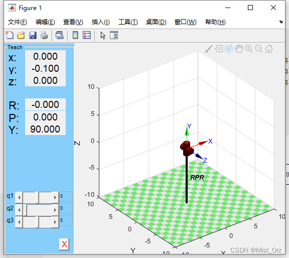
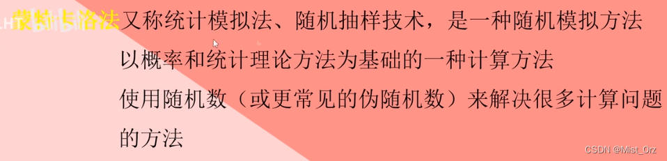
Monte Carlo method of work domain analysis
〇Monte Carlo
code
%定义D-H参数
a2= 0.420;
a3= 0.375;
d2= 0.138+0.024;
d3=-0.127-0.024;
d4= 0.114+0.021;
d5= 0.114+0.021;
d6= 0.090+0.021;


%定义出XYZ的坐标值。
for i=1:100000
theta1=-pi   +2*pi*rand;
theta2=0     +2*pi*rand;
theta3=-(5/6)*pi+(5/3)*pi*rand;
theta4=-pi    +2*pi*rand;
theta5=-pi   +2*pi*rand;
theta6=-pi    +2*pi*rand;

x(i)= a2*cos(theta1)*cos(theta2)+a3*cos(theta1)*cos(theta2+theta3)-d5*cos(theta1)*sin(theta2+theta3+theta4)-sin(theta1)*(d2+d3+d4)-d6*(cos(theta5)*sin(theta1)-cos(theta1)*cos(theta2+theta3+theta4)*sin(theta5));
y(i)=d6*(cos(theta1)*cos(theta5)+cos(theta2+theta3+theta4)*sin(theta1)*sin(theta5))+a3*sin(theta1)*cos(theta2+theta3)-d5*sin(theta1)*sin(theta2+theta3+theta4)+cos(theta1)*(d2+d3+d4)+a2*cos(theta2)*sin(theta1);
z(i)=-a3*sin(theta2+theta3)-a2*sin(theta2)-d5*cos(theta2+theta3+theta4)-d6*sin(theta5)*sin(theta2+theta3+theta4);
end
plot3(x,y,z,'b.','MarkerSize',0.5)
operation result

robot dynamics
〇Equations related to kinetics in the toolbox
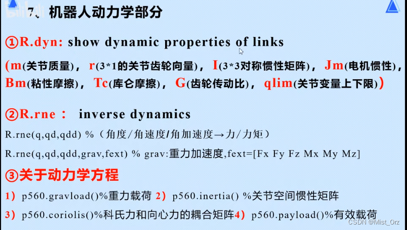
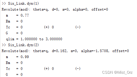
View model dynamics parameters R.dyn()
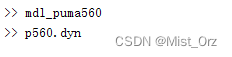
Then it will display the parameters
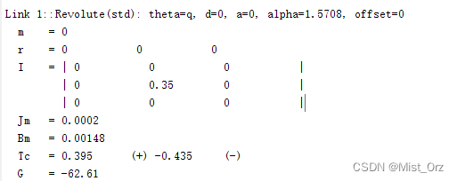
2-6 of each joint slightly
It is also possible to display parameters for individual joints
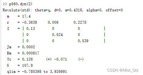
or

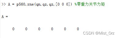
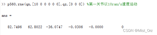
Inverse dynamics R.rne()
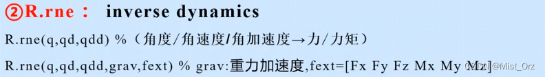
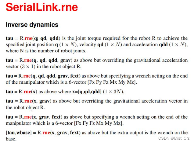
〇 Example
Kinetic equations
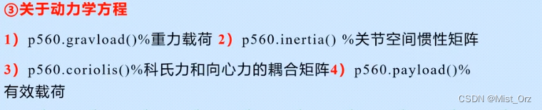


Gravity Load R.gravload()
Calculate the gravity load, the parameter is the joint position, and the result is a vector

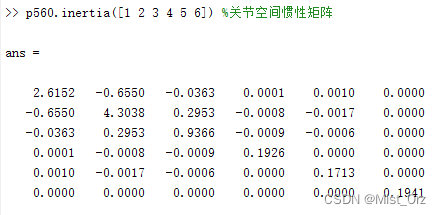
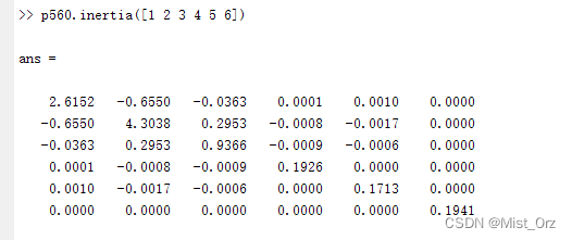
Joint space inertia matrix R.inertia()
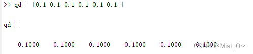
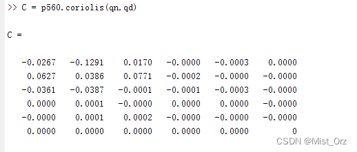
Coriolis force and centripetal force coupling matrix R.coriolis()
First give a speed
qn is the current position in the model
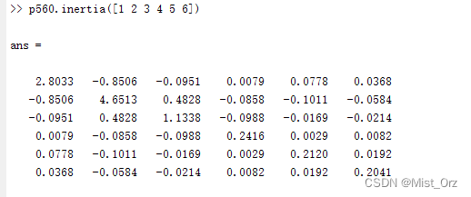
Calculate payload R.payload()
First calculate the inertia matrix without loading,
load the payload

and then calculate the inertia matrix, and find that the value has changed
forward kinetics
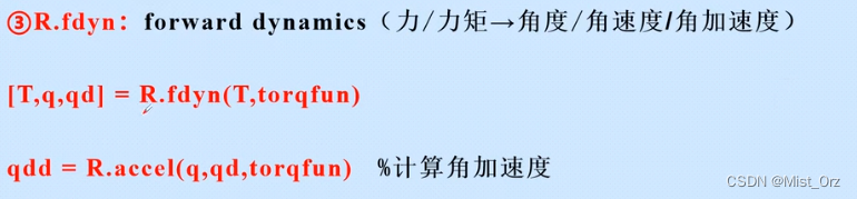
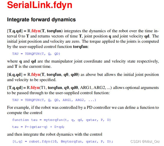
〇 Example
mdl_puma560;
torqfun = [1 2 3 4 5 6];
p560 = p560.nofriction();%没有摩擦的动力学模型,加快求解速度
[T,q,qd] = p560.fdyn(1,torqfun)
for kk = 1:65
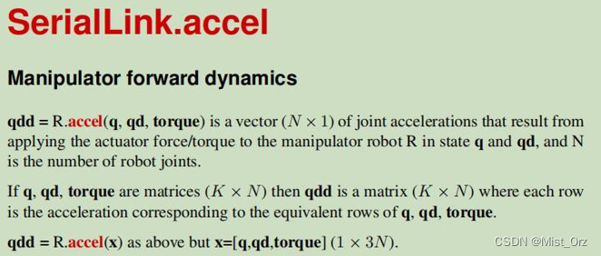
qdd(kk,:) = p560.accel(q(kk,:),qd(kk,:),torqfun);
end
Normally, the acceleration of the joint can be calculated
, but an error is reported.
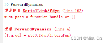
After checking, it seems that the new version of the fdyn() function is a bit different
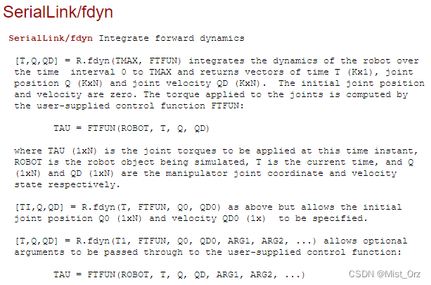
.
Assign dynamic parameters to the robot
First build the DH model
L(1)= Link([0 0 0 0],'modified');
L(2)= Link([0 0.138+0.024 0 -pi/2],'modified');
L(3)= Link([0 -0.127-0.024 0.420 0], 'modified');
L(4)= Link([0 0.114+0.021 0.375 0],'modified');
L(5)= Link([0 0.114+0.021 0 -pi/2],'modified');
L(6)= Link([0 0.090+0.021 0 pi/2],'modified');

Six_Link=SerialLink(L,'name','sixlink');
Then follow the documentation to add the kinetic parameters
L(1).m = 0.77;
L(2).m = 0.99;
L(1).qlim = [1,3];
Then look at the kinetic parameters