Abstract: Merge sort and quick sort are two slightly complicated sorting algorithms. They both use the idea of divide and conquer. The codes are implemented through recursion, and the process is very similar. The key to understanding merge sort is to understand the recursion formula and the merge() merge function.
This article is shared from Huawei Cloud Community " Eight Sorting Algorithms in Simple Ways ", author: Embedded Vision.
Merge sort and quick sort are two slightly complicated sorting algorithms. They both use the idea of divide and conquer, and the code is implemented through recursion. The process is very similar. The key to understanding merge sort is to understand the recursion formula and the merge() merge function.
One, bubble sort (Bubble Sort)
Sorting algorithm is a kind of algorithm that programmers must understand and be familiar with. There are many kinds of sorting algorithms, such as: bubbling, insertion, selection, fast, merge, counting, cardinality and bucket sorting.
Bubble sort will only operate on two adjacent data. Each bubbling operation will compare two adjacent elements to see if they meet the size relationship requirements, and if not, let them be exchanged. One bubbling will move at least one element to where it should be, and repeat n times to complete the sorting of n data.
Summary: If the array has n elements, in the worst case, n bubbling operations are required.
The C++ code of the basic bubble sort algorithm is as follows:
// 将数据从小到大排序
void bubbleSort(int array[], int n){
 if (n<=1) return;
 for(int i=0; i<n; i++){
 for(int j=0; j<n-i; j++){
 if (temp > a[j+1]){
                temp = array[j]
                a[j] = a[j+1];
                a[j+1] = temp;
 }
 }
 }
}
In fact, the above bubble sorting algorithm can also be optimized. When a certain bubbling operation no longer performs data exchange, it means that the array is already in order, and there is no need to continue to perform subsequent bubbling operations. The optimized code is as follows:
// 将数据从小到大排序
void bubbleSort(int array[], int n){
if (n<=1) return;
for(int i=0; i<n; i++){
// 提前退出冒泡循环发标志位
bool flag = False;
for(int j=0; j<n-i; j++){
if (temp > a[j+1]){
temp = array[j]
a[j] = a[j+1];
a[j+1] = temp;
flag = True; // 表示本次冒泡操作存在数据交换
}
}
if(!flag) break; // 没有数据交换,提交退出
}
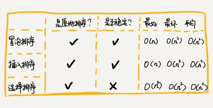
}Features of Bubble Sort :
- The bubbling process only involves the exchange of adjacent elements and only requires a constant level of temporary space, so the space complexity is O(1) O (1), which is an in-place sorting algorithm .
- When there are two adjacent elements of the same size, we do not exchange, and the data of the same size will not change the order before and after sorting, so it is a stable sorting algorithm .
- The worst case and average time complexity are both O(n2) O ( n 2 ), and the best time complexity is O(n) O ( n ).
Second, insertion sort (Insertion Sort)
- The insertion sort algorithm divides the data in the array into two intervals: the sorted interval and the unsorted interval. The initial sorted range has only one element, which is the first element of the array.
- The core idea of the insertion sort algorithm is to take an element of the unsorted range, find a suitable position to insert in the sorted range, and ensure that the data in the sorted range is always in order.
- Repeat this process until the unsorted interval elements are empty, then the algorithm ends.
Insertion sort, like bubble sort, also includes two operations, one is the comparison of elements , and the other is the movement of elements .
When we need to insert a piece of data a into the sorted range, we need to compare the size of a with the elements of the sorted range in order to find a suitable insertion position. After finding the insertion point, we also need to move the order of the elements after the insertion point back one bit, so as to make room for element a to be inserted.
The C++ code implementation of insertion sort is as follows:
void InsertSort(int a[], int n){
 if (n <= 1) return;
 for (int i = 1; i < n; i++) // 未排序区间范围
 {
        key  = a[i]; // 待排序第一个元素
        int j = i - 1; // 已排序区间末尾元素
 // 从尾到头查找插入点方法
 while(key < a[j] && j >= 0){ // 元素比较
            a[j+1] = a[j]; // 数据向后移动一位
            j--;
 }
        a[j+1] = key; // 插入数据
 }
}
Insertion sort features:
- Insertion sorting does not require additional storage space, and the space complexity is O(1) O (1), so insertion sorting is also an in-place sorting algorithm.
- In insertion sorting, for elements with the same value, we can choose to insert the elements that appear later to the back of the elements that appear before, so that the original front and rear order can be kept unchanged, so insertion sort is a stable sorting algorithm.
- The worst case and average time complexity are both O(n2) O ( n 2 ), and the best time complexity is O(n) O ( n ).
Three, selection sort (Selection Sort)
The implementation idea of the selection sorting algorithm is somewhat similar to insertion sorting, and it is also divided into sorted intervals and unsorted intervals. But the selection sort will find the smallest element from the unsorted interval every time, and put it at the end of the sorted interval.
The time complexity of the best case, worst case and average case of selection sorting is O(n2) O ( n 2), which is an in-place sorting algorithm and an unstable sorting algorithm .
The C++ code for selection sort is implemented as follows:
void SelectSort(int a[], int n){
 for(int i=0; i<n; i++){
        int minIndex = i;
 for(int j = i;j<n;j++){
 if (a[j] < a[minIndex]) minIndex = j;
 }
 if (minIndex != i){
            temp = a[i];
            a[i] = a[minIndex];
            a[minIndex] = temp;
 }
 }
}
Bubble insertion selection sort summary
The implementation codes of these three sorting algorithms are very simple, and they are very efficient for sorting small-scale data. However, when sorting large-scale data, the time complexity is still a bit high, so it is more inclined to use a sorting algorithm with a time complexity of O(nlogn) O ( nlogn ).
Certain algorithms depend on certain data structures. The above three sorting algorithms are all implemented based on arrays.
Fourth, merge sort (Merge Sort)
The core idea of merge sort is relatively simple. If we want to sort an array, we first divide the array into front and back parts from the middle, then sort the front and back parts separately, and then merge the sorted two parts together , so that the whole array is in order.
Merge sort uses the idea of divide and conquer. Divide and conquer, as the name suggests, is to divide and conquer, decomposing a big problem into small sub-problems to solve. When the small sub-problems are solved, the big problem is also solved.
The divide-and-conquer idea is somewhat similar to the recursive idea, and the divide-and-conquer algorithm is generally implemented with recursion. Divide and conquer is a processing idea for solving problems, and recursion is a programming technique, and the two do not conflict.
Knowing that merge sorting uses divide-and-conquer thinking, and divide-and-conquer thinking is generally implemented using recursion, the next focus is how to use recursion to implement merge sorting . The skill of writing recursive code is to analyze the problem to get the recursive formula, then find the termination condition, and finally translate the recursive formula into recursive code. Therefore, if you want to write the code for merge sort, you must first write the recursive formula for merge sort .
递推公式:
merge_sort(p…r) = merge(merge_sort(p…q), merge_sort(q+1…r))
终止条件:
p >= r 不用再继续分解,即区间数组元素为 1
The pseudo code for merge sort is as follows:
merge_sort(A, n){
 merge_sort_c(A, 0, n-1)
}
merge_sort_c(A, p, r){
 // 递归终止条件
 if (p>=r) then return
 // 取 p、r 中间的位置为 q
    q = (p+r)/2
 // 分治递归
 merge_sort_c(A[p, q], p, q)
 merge_sort_c(A[q+1, r], q+1, r)
 // 将A[p...q]和A[q+1...r]合并为A[p...r]
 merge(A[p...r], A[p...q], A[q+1...r])
}
4.1, Merge sort performance analysis
1. Merge sort is a stable sorting algorithm . Analysis: The merge_sort_c() function in the pseudo-code only decomposes the problem and does not involve moving elements and comparing sizes. The real element comparison and data movement are in the merge() function part. In the process of merging, the order of elements with the same value is guaranteed to remain unchanged before and after merging. Merge sort sorting is a stable sorting algorithm.
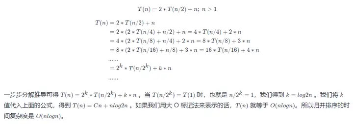
2. The execution efficiency of merge sort has nothing to do with the degree of order of the original array to be sorted, so its time complexity is very stable. Whether it is the best case, the worst case, or the average case, the time complexity is O ( nlogn) O ( nlogn ). Analysis: Not only can the recursive solution problem be written as a recursive formula, but the time complexity of the recursive code can also be written as a recursive formula:
3. The space complexity is O(n) . Analysis: The space complexity of recursive code does not add up like the time complexity. Although each merging operation of the algorithm needs to apply for additional memory space, after the merging is completed, the temporarily opened memory space is released. At any time, the CPU will only have one function executing, and therefore only one temporary memory space in use. The maximum temporary memory space will not exceed the size of n data, so the space complexity is O(n) O ( n ).
Five, quick sort (Quicksort)
The idea of quicksort is this: if we want to sort a set of data with subscripts from p to r in the array, we choose any data between p and r as the pivot (partition point ) . We traverse the data between p and r, put the data smaller than the pivot on the left, put the data larger than the pivot on the right, and put the pivot in the middle. After this step, the data between the array p and r is divided into three parts. The data between p and q-1 in the front is smaller than the pivot, the middle is the pivot, and the data between q+1 and r is greater than the pivot.
According to the idea of divide and conquer and recursion, we can recursively sort the data with subscripts from p to q-1 and the data with subscripts from q+1 to r until the interval is reduced to 1, which means that all The data are all in order.
The recursion formula is as follows:
递推公式:
quick_sort(p,r) = quick_sort(p, q-1) + quick_sort(q, r)
终止条件:
p >= r
Merge sort and quick sort summary
Merge sort and quick sort are two slightly complicated sorting algorithms. They both use the idea of divide and conquer, and the code is implemented through recursion. The process is very similar. The key to understanding merge sort is to understand the recursion formula and the merge() merge function. In the same way, the key to understanding quicksort is to understand the recursive formula, as well as the partition() partition function.
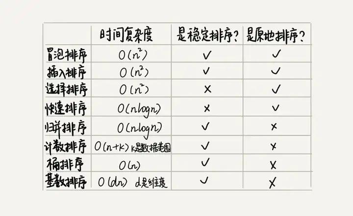
In addition to the above 5 sorting algorithms, there are 3 linear sorting algorithms whose time complexity is O(n) O ( n ) : bucket sorting, counting sorting, and radix sorting. The performance of these eight sorting algorithms is summarized in the following figure:
References
- Sorting (Part 1): Why is insertion sort more popular than bubble sort?
- Sorting (below): How to find the Kth largest element in O(n) with the idea of quick sort?
Click to follow and learn about Huawei Cloud's fresh technologies for the first time~