Top 10 commonly used sorting algorithms (algorithm analysis + animation demonstration)

Various commonly used sorting algorithms

Algorithm overview

Algorithm classification

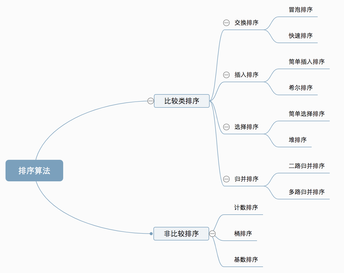
The ten common sorting algorithms can be divided into two broad categories:

• Comparison sorting : The relative order of elements is determined by comparison. Since its time complexity cannot exceed O(nlogn), it is also called nonlinear time comparison sorting.
• Non-comparative sorting : The relative order of elements is not determined by comparison. It can break through the lower bound of comparison-based sorting and run in linear time, so it is also called linear time non-comparative sorting.

​

​

algorithmic complexity

Related concepts

• Stable : If a is originally in front of b, and a=b, a is still in front of b after sorting.
• Unstable : If a is originally in front of b, and a=b, a may appear behind b after sorting.
• Time complexity : The total number of operations on sorted data. It reflects the regularity of the number of operations when n changes.
• Space complexity: refers to the algorithm in the computer

It is a measure of the storage space required for internal execution, and it is also a function of the data size n.

1. Bubble Sort

Bubble sort is a simple sorting algorithm. It iteratively walks through the array to be sorted, comparing two elements at a time and swapping them if they are in the wrong order. The work of visiting the sequence is repeated until there is no need to exchange, that is to say, the sequence has been sorted. The name of this algorithm comes from the fact that the smaller elements will slowly "float" to the top of the sequence through exchange.

1.1 Algorithm description

• Compare adjacent elements. If the first is greater than the second, swap them both;
• Do the same for each pair of adjacent elements, from the first pair at the beginning to the last pair at the end, so the element at the end should be the largest number;
• Repeat the above steps for all elements except the last one;
• Repeat steps 1~3 until sorting is complete.

1.2 Animation presentation

​

1.3 Code implementation

C/C++ implementation:

//冒泡排序 
void bubble_sort(int a[], int n) {//n为a[]的实际长度-1，例如a[4]={3,2,9,10} n为3
    int i,j,tem;
     for (i=0; i<n; i++) 
       for (j=0; j<n-i; j++) //如果左边大于右边则将他们调换位置 
         if (a[j] > a[j+1])tem=a[j],a[j]=a[j+1],a[j+1]=tem;
}

Java implementation:

	//冒泡排序算法
	private static void bubble_sort(int a[], int n) {//n为a[]的实际长度-1，例如a[4]={3,2,9,10} n为3
	     for (int i=0; i<n; i++) 
	       for (int j=0; j<n-i; j++) //如果左边大于右边则将他们调换位置 
	         if (a[j] > a[j+1]) {
	        	 int tem=a[j];a[j]=a[j+1];a[j+1]=tem;
	         }
	}

2. Selection Sort

Selection sort (Selection-sort) is a simple and intuitive sorting algorithm. How it works: first find the smallest (largest) element in the unsorted sequence, store it at the beginning of the sorted sequence, then continue to find the smallest (largest) element from the remaining unsorted elements, and then put it in the sorted sequence end of . And so on until all elements are sorted.

2.1 Algorithm description

The direct selection and sorting of n records can obtain ordered results through n-1 direct selection and sorting. The specific algorithm is described as follows:

• Initial state: the unordered area is R[1...n], and the ordered area is empty;
• When the i-th sorting (i=1,2,3...n-1) starts, the current ordered area and unordered area are R[1...i-1] and R(i...n) respectively. This sorting process selects the record R[k] with the smallest key from the current unordered area, and exchanges it with the first record R in the unordered area, so that R[1...i] and R[i+1... n) respectively become a new ordered area in which the number of records increases by 1 and a new disordered area in which the number of records decreases by 1;
• The n-1 trip is over, and the array is sorted.

2.2 Animation presentation

2.3 Code implementation

C/C++ implementation:

//选择排序  
void selection_sort (int a[], int n) {//n为a[]的实际长度-1，例如a[4]={3,2,9,10} n为3
   
   for(int i=0;i<=n;i++) 
    for(int j=i+1;j<=n;j++)
     if(a[i]>a[j]){int tem=a[i];a[i]=a[j];a[j]=tem;}
}

Java implementation:

//选择排序  
	public static void selection_sort (int a[], int n) {
    
    //n为a[]的实际长度-1，例如a[4]={3,2,9,10} n为3
	   for(int i=0;i<=n;i++) //每次选出第i小的数 
	    for(int j=i+1;j<=n;j++)//与后面没排序的依次比较 选出当前最小的数 
	     if(a[i]>a[j]){
    
    int tem=a[i];a[i]=a[j];a[j]=tem;}
	}

2.4 Algorithm analysis

One of the most stable sorting algorithms, because no matter what data is entered, it has a time complexity of O(n2), so when it is used, the smaller the data size, the better. The only advantage may be that it does not take up additional memory space. Theoretically speaking, selection sorting may also be the sorting method that most people usually think of when sorting.

3. Insertion Sort

The algorithm description of Insertion-Sort is a simple and intuitive sorting algorithm. It works by constructing an ordered sequence, and for unsorted data, scans from the back to the front in the sorted sequence, finds the corresponding position and inserts it.

3.1 Algorithm description

Generally speaking, insertion sort is implemented on arrays using in-place. The specific algorithm is described as follows:

• Starting from the first element, the element can be considered sorted;
• Take out the next element and scan from back to front in the sorted element sequence;
• If the element (sorted) is larger than the new element, move the element to the next position;
• Repeat step 3 until you find the position where the sorted element is less than or equal to the new element;
• After inserting a new element at that position;
• Repeat steps 2~5.

3.2 Animation presentation

3.2 Code implementation

C/C++ implementation

//插入排序  
void insertion_sort (int a[], int n) {
    
    //n为a[]的实际长度-1，例如a[4]={3,2,9,10} n为3
     int i,j,tem;//tem 中间临时变量 
	 for (i=1; i<=n; i++) {
    
    
//当前i与前(i-1)个做比较如果当前i元素小于前(i-1)个,则第(i-1)个向挪一位 
     for (tem=a[i],j=i-1;j>=0&&tem<a[j];j--)a[j+1]=a[j]; 
        a[j+1]=tem;//确定当前i应该到的位置 
    }
}

Java implementation

//插入排序算法：
	private static void insertion_sort (int a[], int n) {
    
    //n为a[]的实际长度-1，例如a[4]={3,2,9,10} n为3
	     int i,j,tem;//中间临时变量 
		 for (i=1; i<=n; i++) {
    
    
	//当前i与前(i-1)个做比较如果当前i元素小于前(i-1)个,则第(i-1)个向挪一位 
	     for (tem=a[i],j=i-1;j>=0&&tem<a[j];j--)a[j+1]=a[j]; 
	        a[j+1]=tem;//确定当前i应该到的位置 
	    }
	}
	

3.4 Algorithm analysis

In the implementation of insertion sorting, in-place sorting is usually used (that is, sorting that only needs to use O(1) extra space), so in the process of scanning from back to forward, it is necessary to repeatedly move the sorted elements backwards step by step , providing insertion space for the newest element.

4. Shell Sort

Invented by Shell in 1959, the first sorting algorithm to break through O(n2) is an improved version of simple insertion sort. It differs from insertion sort in that it compares elements that are farther away first. Hill sort is also called shrinking incremental sort .

4.1 Algorithm description

First divide the entire record sequence to be sorted into several subsequences for direct insertion sorting respectively. The specific algorithm description:

• Choose an incremental sequence t1, t2, ..., tk, where ti>tj, tk=1;
• According to the incremental sequence number k, sort the sequence k times;
• For each sorting, according to the corresponding increment ti, the column to be sorted is divided into several subsequences of length m, and direct insertion sorting is performed on each sublist respectively. Only when the increment factor is 1, the entire sequence is treated as a table, and the length of the table is the length of the entire sequence.

4.2 Animation presentation

4.3 Code implementation

 C/C++ 实现：

//希尔排序 
void shell_sort(int a[],int n){
    
    //n为a[]的实际长度-1，例如a[4]={3,2,9,10} n为3
  for(int d=n/2;d>0;d/=2)//d 为增量 
	 for(int i=d;i<=n;i++){
    
    
	 	 int j=i;
	 	 int tem=a[j];//j-d 代表 当前j的前一个元素（当前同一个分组） 
		  while(j-d>=0&&a[j-d]>tem) a[j]=a[j-d],j=j-d;// 插入排序的方法 
		  a[j]=tem;
	 }
}

Java implementation:

	//希尔排序 
	private static void shell_sort(int a[],int n){
    
    
	  for(int d=n/2;d>0;d/=2)//d 为增量 
		 for(int i=d;i<=n;i++){
    
    
		 	 int j=i;
		 	 int tem=a[j];//j-d 代表 当前j的前一个元素（当前同一个分组） 
			  while(j-d>=0&&a[j-d]>tem) {
    
    a[j]=a[j-d];j=j-d;}// 插入排序的方法 
			  a[j]=tem;
		 }
	}

4.4 Algorithm analysis

The core of Hill sorting lies in the setting of the interval sequence. The interval sequence can be set in advance, or the interval sequence can be defined dynamically. The algorithm for dynamically defining interval sequences was proposed by Robert Sedgewick, co-author of Algorithms (4th Edition).

5. Merge Sort

Merge sort is an efficient sorting algorithm based on the merge operation. This algorithm is a very typical application of Divide and Conquer. Combine the ordered subsequences to obtain a completely ordered sequence; that is, first make each subsequence in order, and then make the subsequence segments in order. Merging two sorted lists into one sorted list is called a 2-way merge.

5.1 Algorithm description

• Divide an input sequence of length n into two subsequences of length n/2;
• Use merge sort for the two subsequences respectively;
• Merges two sorted subsequences into a final sorted sequence.

5.2 Animation presentation

5.3 Code implementation

C/C++ implementation:

//归并排序
void merge_core(int a[],int l,int mid,int r){
    
    //合并数组 
	int k=0,i=l,j=mid+1;
	int *tem=(int*)malloc(sizeof(int)*(r-l+1));//开临时中间数组 
	// 执行合并 谁小谁先进tem    两个组比大小 
	while(i<=mid||j<=r)tem[k++]=((a[i]<a[j]&&i<=mid)||j>r)?a[i++]:a[j++]; 
    while(k--)a[r--]=tem[k]; free(tem);//清除空间 
}
void merge_sort(int a[],int l,int r){
    
    
	if(r>l){
    
    
	int mid=(l+r)>>1;//取中间 一分为二 
	merge_sort(a,l,mid); 
	merge_sort(a,mid+1,r);
	merge_core(a,l,mid,r);//合并 
	}
} 

Java implementation:

   //归并排序
	private static void mergeSort(int a[],int l,int r){
    
    
		if(r>l){
    
    
		int mid=(l+r)>>1;//取中间 一分为二 
		mergeSort(a,l,mid); 
		mergeSort(a,mid+1,r);
		mergeCore(a,l,mid,r);//合并 
		}
	}
	private static void  mergeCore(int a[],int l,int mid,int r){
    
    //合并数组 
		int k=0,i=l,j=mid+1;
		int tem[]=new int[r-l+2];//开临时中间数组 
		// 执行合并 谁小谁先进   两个组比大小 
		while(i<=mid||j<=r)tem[k++]=(j>r||(i<=mid&&a[i]<a[j]))?a[i++]:a[j++]; 
	    while(k!=0)a[r--]=tem[--k]; 
	}

5.4 Algorithm analysis

Merge sort is a stable sorting method. Like selection sort, the performance of merge sort is not affected by the input data, but the performance is much better than selection sort, because it is always O(nlogn) time complexity. The cost is that additional memory space is required.

6. Quick Sort

The basic idea of ​​quick sorting: the records to be sorted are separated into two independent parts by one-pass sorting, and the keywords of one part of the records are smaller than the keywords of the other part, then the two parts of the records can be sorted separately to achieve The whole sequence is in order.

6.1 Algorithm description

Quicksort uses a divide-and-conquer method to divide a string (list) into two sub-strings (sub-lists). The specific algorithm is described as follows:

• Pick an element from the sequence, called the "pivot" (pivot);
• Reorder the sequence, all elements smaller than the reference value are placed in front of the reference value, and all elements larger than the reference value are placed behind the reference value (the same number can go to either side). After this partition exits, the benchmark is in the middle of the sequence. This is called a partition operation;
• Recursively sort subarrays with elements less than the base value and subarrays with elements greater than the base value.

6.2 Animation presentation

6.3 Code implementation

C/C++ implementation:

int mp(int a[], int l, int r) {
    
    
    int p = a[r];
    while (l<r) {
    
    
		while (l<r && p>a[l])l++;//从左向右寻找比标准p大的数
		if(l<r) a[r--]=a[l];//找到了就放到最右边,比标准p大就应该在右边  
        while (l<r && p<a[r])r--;//从右向左寻找比标准p小的数
        if(l<r) a[l++]=a[r];//找到就放到最左边,比标准p大就应该在左边 
    }
    a[r]=p;
    return r; 
}
//快速排序 
void quick_sort (int a[], int l, int r) {
    
    //r为a[]的实际长度-1，例如a[4]={3,2,9,10} l为0 r为3
    if (l < r) {
    
    
        int q = mp(a, l, r);//找到标准应该在的位置 
        quick_sort(a, l, q-1);//根据标准的位置分为左边部分 
        quick_sort(a, q+1, r);//根据标准的位置分为右边部分 
    }
}

Java implementation:

	//快速排序
    private static void quickSort(int[] a, int l, int r) {
    
    //r为a[]的实际长度-1，例如a[4]={3,2,9,10} l为0 r为3
		if(l<r) {
    
    
			     int p=mpSort(a,l,r);//找到标准应该在的位置 
			     quickSort(a,l,p-1);//根据标准的位置分为左边部分 
			     quickSort(a,p+1,r);//根据标准的位置分为右边部分
		}
	}
	
	private static int mpSort(int[] a, int l, int r) {
    
    
		int p=a[r];
		while(l<r) {
    
    
			while(l<r&&p>a[l])l++;//从左向右寻找比标准p大的数
			if(l<r)a[r--]=a[l];//找到了就放到最右边,比标准p大就应该在右边  
			while(l<r&&p<a[r])r--;//从右向左寻找比标准p小的数
			if(l<r)a[l++]=a[r];//找到就放到最左边,比标准p大就应该在左边 
		} a[l]=p;
		return l;
	}

6.4 Algorithm analysis

The time complexity of the quick sort algorithm has a great relationship with the value of each standard data element. If the standard elements selected each time can equally divide the length of the two sub-arrays, such a quick sorting process is a complete binary tree structure. (That is, each node divides the current array into two array nodes of equal size, and the number of decompositions of the root node of the n-element array constitutes a complete binary tree). At this time, the number of decompositions is equal to the depth log2n of the complete binary tree. No matter how the array is divided in each quick sorting process, the total number of comparisons is close to n-1 times, so the time complexity of the quick sorting algorithm is O(nlog2n) in the best case. : The worst case of the quick sort algorithm is that the data elements are all in order. At this time, the number of times the root node of the data element array needs to be divided constitutes a binary degenerate tree (that is, a single-branch binary tree), and a binary degenerate tree The depth is n. So the worst case time complexity of quicksort algorithm is O(n2). In general, the distribution of standard element values ​​is random, and the depth of such a binary tree is close to log2n, so the average (or expected) time complexity of the quick sort algorithm is O(nlog2n)

7. Heap Sort

Heapsort (Heapsort) refers to a sorting algorithm designed using the data structure of the heap. Stacking is a structure that approximates a complete binary tree, and at the same time satisfies the nature of stacking: that is, the key value or index of a child node is always smaller (or larger) than its parent node.

7.1 Algorithm description

• Build the initial sequence of keywords to be sorted (R1, R2....Rn) into a large top heap, which is the initial unordered area;
• Exchange the top element R[1] with the last element R[n], and get a new unordered area (R1, R2,...Rn-1) and a new ordered area (Rn), and satisfy R [1,2...n-1]<=R[n];
• Since the new heap top R[1] after the exchange may violate the nature of the heap, it is necessary to adjust the current unordered area (R1, R2,...Rn-1) to a new heap, and then combine R[1] with the unordered area again The last element of the region is exchanged to obtain a new disordered region (R1, R2....Rn-2) and a new ordered region (Rn-1, Rn). This process is repeated until the number of elements in the ordered area is n-1, and the entire sorting process is completed.

7.2 Animation presentation

7.3 Code implementation

C/C++ implementation:

//大顶堆 
void max_heapify(int a[], int l, int r) {
    
    
    int f= l;//建立父节点指标和子节点指标
    int s= f*2+1;
    while (s <=r) {
    
     //若子节点指标在范围内才做比较
        if (s+1<=r&&a[s]<a[s+1])s++;//先比较两个子节点大小，选择最大的
        if (a[f]<a[s]){
    
    //如果父节点小于子节点代表需调整，交换父子内容再继续子节点和孙节点比较
            int tem=a[f];a[f]=a[s];a[s]=tem;
            f=s;
            s=f*2+1;//交换父子内容再继续子节点和孙节点比较
        }else return;//调整好了直接跳出  
    }
}
//堆排序 
void heap_sort(int a[], int n) {
    
    
    for (int i=n/2; i>= 0; i--)max_heapify(a,i,n);//i从最後一个父节点开始调整
    //先将第一个元素和已排好元素前一位做交换，再重新调整，直到排序完毕
    for (int i=n; i>0;i--) {
    
    
        int tem=a[0];a[0]=a[i];a[i]=tem;
        max_heapify(a,0,i-1);
    }
}

Java implementation:

	//堆排序 
	private static void heapSort(int a[], int n) {
    
    
	    for (int i=n/2; i>= 0; i--)maxHeapify(a,i,n);//i从最後一个父节点开始调整
	    //先将第一个元素和已排好元素前一位做交换，再重新调整，直到排序完毕
	    for (int i=n; i>0;i--) {
    
    
	        int tem=a[0];a[0]=a[i];a[i]=tem;
	        maxHeapify(a,0,i-1);
	    }
	}
	//大顶堆 
		private static void maxHeapify(int a[], int l, int r) {
    
    
		    int f= l;//建立父节点指标和子节点指标
		    int s= f*2+1;
		    while (s <=r) {
    
     //若子节点指标在范围内才做比较
		        if (s+1<=r&&a[s]<a[s+1])s++;//先比较两个子节点大小，选择最大的
		        if (a[f]<a[s]){
    
    //如果父节点小于子节点代表需调整，交换父子内容再继续子节点和孙节点比较
		            int tem=a[f];a[f]=a[s];a[s]=tem;
		            f=s;
		            s=f*2+1;//交换父子内容再继续子节点和孙节点比较
		        }else return;//调整好了直接跳出 
		    }
		}
	

7.4 Algorithm analysis

Heap sorting is an unstable sorting algorithm. For a sequence of n elements, to construct a heap process, the number of elements that need to be traversed is O(n), and the number of adjustments for each element is O(log2n), so the complexity of constructing a heap is O(nlog2n). The number of iterations to replace the first and last elements of the set to be sorted is O(n), and the number of adjustments after each replacement is O(log2n), so the complexity of the iterative operation is O(nlog2n). It can be seen that the time complexity of heap sorting is O(nlog2n), and the sorting process belongs to in-place sorting, which does not require additional storage space, so the space complexity is O(1).

8. Counting Sort

Counting sorting is not a sorting algorithm based on comparison. Its core is to convert the input data value into a key and store it in the additional array space. As a sort of linear time complexity, counting sort requires that the input data must be integers with a certain range.

8.1 Algorithm description

• Find the largest and smallest elements in the array to be sorted;
• Count the number of occurrences of each element whose value is i in the array, and store it in the i-th item of the array C;
• Accumulate all counts (starting from the first element in C, each item is added to the previous item);
• Fill the target array in reverse: put each element i in the C(i)th item of the new array, and subtract 1 from C(i) every time an element is placed.

8.2 Animation presentation

8.3 Code implementation

C/C++ implementation:

 //计数排序 
 void counting_sort(int a[],int n){
    
    
 	  int max_num=0,k=0; //获取最大值 
	 for(int i=1;i<=n;i++)if(a[i]>a[max_num])max_num=i;max_num=a[max_num];
     int count[max_num+1]; memset(count,0,sizeof(count));//初始化计数数组 
     for(int i=0;i<=n;i++)count[a[i]]++;//开始计数 
     for(int i=0;i<=max_num;i++){
    
     //排序 
	   while(count[i]--)a[k++]=i;//到正确的位置 
     }
 } 

Java implementation:

private static void counting_sort(int a[],int n){
    
    
		     int max_num=0,k=0; //获取最大值 
			 for(int i=1;i<=n;i++)if(a[i]>a[max_num])max_num=i;
			        max_num=a[max_num];
		     int []count=new int[max_num+1]; //初始化计数数组 
		     for(int i=0;i<=n;i++)count[a[i]]++;//开始计数 
		     for(int i=0;i<=max_num;i++){
    
     //排序 
			   while(0<count[i]--)a[k++]=i;//到正确的位置 
		     }
		 }
		

8.4 Algorithm analysis

Counting sort is a stable sorting algorithm. When the input elements are n integers between 0 and k, the time complexity is O(n+k), the space complexity is also O(n+k), and its sorting speed is faster than any comparison sorting algorithm. Counting sort is an efficient sorting algorithm when k is not very large and the sequences are relatively concentrated.

9. Bucket Sort

Bucket sort is an upgraded version of counting sort. It makes use of the mapping relationship of functions, and the key to high efficiency lies in the determination of this mapping function. The working principle of bucket sort (Bucket sort): Assuming that the input data is uniformly distributed, the data is divided into a limited number of buckets, and each bucket is sorted separately (it is possible to use other sorting algorithms or continue to use recursively) bucket sort).

9.1 Algorithm description

• Set a quantitative array as an empty bucket;
• Traverse the input data and put the data one by one into the corresponding bucket;
• Sort each bucket that is not empty;
• Concatenate sorted data from non-empty buckets.

9.2 Animation presentation

9.3 Code implementation

function bucketSort(arr, bucketSize) {
    
    
    if (arr.length === 0) {
    
    
      return arr;
    }
    var i;
    var minValue = arr[0];
    var maxValue = arr[0];
    for (i = 1; i < arr.length; i++) {
    
    
      if (arr[i] < minValue) {
    
    
          minValue = arr[i];               // 输入数据的最小值
      }else if (arr[i] > maxValue) {
    
    
          maxValue = arr[i];               // 输入数据的最大值
      }
    }
    // 桶的初始化
    var DEFAULT_BUCKET_SIZE = 5;           // 设置桶的默认数量为5
    bucketSize = bucketSize || DEFAULT_BUCKET_SIZE;
    var bucketCount = Math.floor((maxValue - minValue) / bucketSize) + 1;  
    var buckets =new Array(bucketCount);
    for (i = 0; i < buckets.length; i++) {
    
    
        buckets[i] = [];
    }
    // 利用映射函数将数据分配到各个桶中
    for (i = 0; i < arr.length; i++) {
    
    
        buckets[Math.floor((arr[i] - minValue) / bucketSize)].push(arr[i]);
    }

    arr.length = 0;
    for (i = 0; i < buckets.length; i++) {
    
    
        insertionSort(buckets[i]);                     // 对每个桶进行排序，这里使用了插入排序
        for (var j = 0; j < buckets[i].length; j++) {
    
    
            arr.push(buckets[i][j]);                     
        }
    }
    return arr;
}

9.4 Algorithm analysis

Bucket sorting uses linear time O(n) in the best case. The time complexity of bucket sorting depends on the time complexity of sorting data between buckets, because the time complexity of other parts is O(n). Obviously, the smaller the buckets are divided, the less data there is between each bucket, and the less time it takes to sort. But the corresponding space consumption will increase.

10. Radix Sort

Cardinality sorting is to sort according to the low order first, and then collect; then sort according to the high order, and then collect; and so on, until the highest order. Sometimes some attributes are prioritized, first sorted by low priority, and then sorted by high priority. The final order is that the one with the higher priority comes first, and the one with the same high priority and the lower priority comes first.

10.1 Algorithm description

• Obtain the maximum number in the array and obtain the number of digits;
• arr is the original array, each bit is taken from the lowest bit to form a radix array;
• Perform counting sort on radix (using the feature that counting sort is suitable for small range numbers);

10.2 Animation presentation

10.3 Code implementation

var counter = [];
function radixSort(arr, maxDigit) {
    
    
    var mod = 10;
    var dev = 1;
    for (var i = 0; i < maxDigit; i++, dev *= 10, mod *= 10) {
    
    
        for(var j = 0; j < arr.length; j++) {
    
    
            var bucket = parseInt((arr[j] % mod) / dev);
            if(counter[bucket]==null) {
    
    
                counter[bucket] = [];
            }
            counter[bucket].push(arr[j]);
        }
        var pos = 0;
        for(var j = 0; j < counter.length; j++) {
    
    
            var value =null;
            if(counter[j]!=null) {
    
    
                while ((value = counter[j].shift()) !=null) {
    
    
                      arr[pos++] = value;
                }
          }
        }
    }
    return arr;
}

10.4 Algorithm Analysis

Radix sorting is based on sorting separately and collecting separately, so it is stable. However, the performance of radix sorting is slightly worse than that of bucket sorting. Each keyword bucket allocation requires O(n) time complexity, and obtaining a new keyword sequence after allocation requires O(n) time complexity. If the data to be sorted can be divided into d keywords, the time complexity of radix sorting will be O(d*2n). Of course, d is much smaller than n, so it is basically linear.

The space complexity of radix sort is O(n+k), where k is the number of buckets. Generally speaking, n>>k, so the extra space needs about n or so.