数据分析三剑客之 Pandas 基础教程

0.1 先导条件：

import numpy as np
import pandas as pd

1 创建对象：

1.1 Series:

pd.Series 是能够保存任何类型的数据(整数，字符串，浮点数，Python对象等)的一维标记数组。轴标签统称为索引。

• data 参数
• index 索引 索引值必须是唯一的和散列的，与数据的长度相同。 默认np.arange(n)如果没有索引被传递。
• dtype 输出的数据类型 如果没有，将推断数据类型
• copy 复制数据 默认为false

1.1.1 通过列表创建Series：

data = ['1', 'a', 'A', '@', 100, 3.1415926, 'giao',[_ for _ in range(5)], np.nan, '么的对象']  # data可以有多种数据类型
s = pd.Series(data=data,
              index=[1, 2, 3.1415926, 4, [_ for _ in range(3)], 'a', 'B', '*', '这也算', 'index']  # index也一样
              )
print(s)

1                          1
2                          a
3.1415926                  A
4                          @
[0, 1, 2]                100
a                    3.14159
B                       giao
*            [0, 1, 2, 3, 4]
这也算                      NaN
index                   么的对象
dtype: object

1.1.2 通过字典创建Series：

ps = pd.Series({'A': 0, 'index': '*', '索引': [1, '*', 'qwer']})
print(ps)

A                   0
index               *
索引       [1, *, qwer]
dtype: object

1.1.3 为Series对象即索引添加名字：

ps.name = "对象名字"
ps.index.name = "索引名字"
print(ps)

索引名字
A                   0
index               *
索引       [1, *, qwer]
Name: 对象名字, dtype: object

1.2 DataFrame:

pd.DataFrame 是能够保存任何类型的数据(整数，字符串，浮点数，Python对象、Series、另一个DataFrame等)的二维标记数组。有行索引(index)和列索引(columns)。

• data表示要传入的数据 ，包括 ndarray，series，map，lists，dict，constant和另一个DataFrame
• index和columns 行索引和列索引 格式[‘x1’,‘x2’]
• dtype:每列的类型
• copy: 从input输入中拷贝数据。默认是false，不拷贝。

1.2.1 通过NumPy数组创建DataFrame：

df = pd.DataFrame(data=np.random.randn(6, 4),  # 通过numpy创建一个 6×4 的数组
                  index=['index', 2, '索引', 'b',[_ for _ in range(3)], '&'],  # index有6个元素，可以为不同类型
                  columns=['columns', 1, '%', '列']  # conlumns有4个元素，不能为list
                  )
df  # print(df)

	columns	1	%	列
index	0.435026	-0.032693	-0.563487	-0.115501
2	0.140005	0.339203	0.751511	0.508840
索引	-0.083063	0.698902	1.746227	1.169957
b	0.702406	1.115746	0.272275	0.247573
[0, 1, 2]	-0.297025	1.812985	0.990014	-1.267218
&	1.206636	1.556716	0.028735	-0.679610

1.2.2 通过字典创建DataFrame：

df2 = pd.DataFrame({'A': [_ for _ in range(4)],
                    'B': pd.Timestamp('20200317'),
                    'C': pd.Series(1, index=list(range(4)), dtype='float32'),
                    'D': np.array([3]*4, dtype='int32'),
                    'E': pd.Categorical(['test', 'train', 'test', 'train']),
                    'F': 'foo'})
df2  # print(df2)

	A	B	C	D	E	F
0	0	2020-03-17	1.0	3	test	foo
1	1	2020-03-17	1.0	3	train	foo
2	2	2020-03-17	1.0	3	test	foo
3	3	2020-03-17	1.0	3	train	foo

1.2.3 通过嵌套字典创建自定义行列索引的DataFrame：

外面的是列索引，嵌套进去的是行索引

df3 = pd.DataFrame({"第1列": {"第1行": "a", "第2行": "b"},
                    "第2列": {"第1行": "*", "第2行": "?"}}
                   )
df3  # print(df3)

	第1列	第2列
第1行	a	*
第2行	b	?

2 查看数据：

先重新建个表：

df = pd.DataFrame(data=np.arange(1, 25).reshape(6, 4), index=[_ for _ in range(1, 7)], columns=['A', 'B', 'C', 'D'])
df  # print(df)

	A	B	C	D
1	1	2	3	4
2	5	6	7	8
3	9	10	11	12
4	13	14	15	16
5	17	18	19	20
6	21	22	23	24

2.1 查看数据的头和尾：

df.head()  # print(df.head())  # 默认查看前（后）5个

	A	B	C	D
1	1	2	3	4
2	5	6	7	8
3	9	10	11	12
4	13	14	15	16
5	17	18	19	20

df.tail(2)  # print(df.tail(2))  # 也可以指定

	A	B	C	D
5	17	18	19	20
6	21	22	23	24

2.2 查看中间的细节：

2.2.1 查看索引名：

print(df.index)

Int64Index([1, 2, 3, 4, 5, 6], dtype='int64')

2.2.2 查看列名：

print(df.columns)

Index(['A', 'B', 'C', 'D'], dtype='object')

2.2.3 查看所有值：

print(df.values)

[[ 1  2  3  4]
 [ 5  6  7  8]
 [ 9 10 11 12]
 [13 14 15 16]
 [17 18 19 20]
 [21 22 23 24]]

2.2.4 查看行数/列数：

print(df.shape[0])  # 行数
print(df.shape[1])  # 列数

6
4

2.2.5 行/列求和：

print(df.sum(0))  # 行
print(df.sum(1))  # 列

A    66
B    72
C    78
D    84
dtype: int64
1    10
2    26
3    42
4    58
5    74
6    90
dtype: int64

2.2.6 数据类型：

print(df.dtypes)

A    int32
B    int32
C    int32
D    int32
dtype: object

2.3 查看数据的统计信息(describe)：

查看数据按列的统计信息，可显示数据的数量、缺失值、最小最大数、平均值、分位数等信息

df.describe(

    percentiles=None,  #这个参数可以设定数值型特征的统计量，默认是[.25, .5, .75],也就是返回25%，50%，75%数据量时的数字，
                      但是这个可以修改，像这样：df['Parch'].describe(percentiles=[.2,.75, .8]) （但还是有50%时的数据）
    include=None,   
    
    exclude=None

)

df.describe()  # print(df.describe())

	A	B	C	D
count	6.000000	6.000000	6.000000	6.000000
mean	11.000000	12.000000	13.000000	14.000000
std	7.483315	7.483315	7.483315	7.483315
min	1.000000	2.000000	3.000000	4.000000
25%	6.000000	7.000000	8.000000	9.000000
50%	11.000000	12.000000	13.000000	14.000000
75%	16.000000	17.000000	18.000000	19.000000
max	21.000000	22.000000	23.000000	24.000000

2.4 数据转置：

df.T  # print(df.T)

	1	2	3	4	5	6
A	1	5	9	13	17	21
B	2	6	10	14	18	22
C	3	7	11	15	19	23
D	4	8	12	16	20	24

2.5 数据排序：

两种方式：df. sort_index() 和 df.sort_values()

df. sort_index()可以完成和df. sort_values()完全相同的功能，

但python更推荐用只用df. sort_index()对“根据行标签”和“根据列标签”排序，其他排序方式用df.sort_values()。

2.5.1 沿某一轴排序：

df.sort_index(

    axis：0按照行名排序；1按照列名排序,默认为0
    
    level：默认None，否则按照给定的level顺序排列---貌似并不是，文档
    
    ascending：默认True升序排列；False降序排列
    
    inplace：布尔型，是否用排序后的数据框替换现有的数据框，默认否
    
    kind：排序方法，{‘quicksort’, ‘mergesort’, ‘heapsort’}, default ‘quicksort’。似乎不用太关心。
    
    na_position：缺失值默认排在最后{"first","last"}
    
    by：按照某一列或几列数据进行排序

)

df.sort_index(ascending=False)  # print(df.sort_index(ascending=False))

	A	B	C	D
6	21	22	23	24
5	17	18	19	20
4	13	14	15	16
3	9	10	11	12
2	5	6	7	8
1	1	2	3	4

2.5.2 按照值进行排序：

df.sort_values(

    axis：{0 or ‘index’, 1 or ‘columns’}, 默认为0，按照列排序，即纵向排序；如果为1，则是横向排序
    
    by：str or list of str；如果axis=0，那么by="列名"；如果axis=1，那么by="行名"
    
    ascending：布尔型，True则升序，如果by=['列名1','列名2']，则该参数可以是[True, False]，即第一字段升序，第二个降序，默认True
    
    inplace：布尔型，是否用排序后的数据框替换现有的数据框，默认否
    
    kind：排序方法，{‘quicksort’, ‘mergesort’, ‘heapsort’}, 默认 ‘quicksort’，似乎不用太关心...
    
    na_position：{‘first’, ‘last’}, default ‘last’，默认缺失值排在最后面

)

df.sort_values(by='B', ascending=False) # print(df.sort_values(by='B', ascending=False))

	A	B	C	D
6	21	22	23	24
5	17	18	19	20
4	13	14	15	16
3	9	10	11	12
2	5	6	7	8
1	1	2	3	4

3 数据选择：

3.1 数据获取：(基本方法)

3.1.1 根据列名获取某一列的数据：

print("第一列的Series:")  # 根据列名查看某一列的值(返回Series)
print(df['A'])

print("第一列的Series(法2)：")  # 效果同上
print(df.A)

print("第一列的值：")  # 根据列名查看某一列的值(返回numpy.ndarray)
print(df['A'].values)

第一列的Series:
1     1
2     5
3     9
4    13
5    17
6    21
Name: A, dtype: int32
第一列的Series(法2)：
1     1
2     5
3     9
4    13
5    17
6    21
Name: A, dtype: int32
第一列的值：
[ 1  5  9 13 17 21]

3.1.2 切片获取某几行数据：

df[0:3]  # print(df[0:3])  # 按行号切片

	A	B	C	D
1	1	2	3	4
2	5	6	7	8
3	9	10	11	12

df[2:4]  # print( df[2:4])#按行名切片
# 由于这里我的行名是整型，所以按行名切片是的索引不能加引号

	A	B	C	D
3	9	10	11	12
4	13	14	15	16

3.2 根据名称选择数据(loc)：

df.loc查找元素都是根据名称

3.2.1 行名查找：

print(df.loc[1])  # 注意，在这里，行名时整型，那么中括号里的索引也应该是整型，不能加引号

A    1
B    2
C    3
D    4
Name: 1, dtype: int32

3.2.2 切片获取某几行的数据：

其实就是选取所有列，再选择某几行

df.loc[2:3, ]  # print(df.loc[2:3, ])

	A	B	C	D
2	5	6	7	8
3	9	10	11	12

3.2.3 切片获取某几列的数据：

其实就是选取所有行，再选择某几列

df.loc[:, ['A', 'B']]  # print(df.loc[:, ['A', 'B']])

	A	B
1	1	2
2	5	6
3	9	10
4	13	14
5	17	18
6	21	22

3.2.4 获取特定位置的数据：(标量)

就是结合上面两种方法

print(df.loc[1, 'A'])
print(df.at[1, 'A'])  # 效果一样

1
1

3.2.5 获取某几行某几列的数据：(连续)

df.loc[1:3, 'A':'C']  # print(df.loc[1:3, 'A':'C'])

	A	B	C
1	1	2	3
2	5	6	7
3	9	10	11

3.2.6 获取某几行某几列的数据：(离散)

df.loc[[1, 3], ['A', 'C']]# print(df.loc[[1, 3], ['A', 'C']])

	A	C
1	1	3
3	9	11

3.2.7 降维返回某一行指定列的数据：

print(df.loc[2, ['B', 'C']])

B    6
C    7
Name: 2, dtype: int32

3.3 根据位置选择数据(iloc)：

df.iloc查找元素都是根据位置(下标/索引)

3.3.1 行号查找：

print(df.iloc[0])

A    1
B    2
C    3
D    4
Name: 1, dtype: int32

3.3.2 切片获取某几行的数据：

df.iloc[3:5, :]  # print(df.iloc[3:5,:])

	A	B	C	D
4	13	14	15	16
5	17	18	19	20

3.3.3 切片获取某几列的数据：

df.iloc[:, 2:4]  # print(df.iloc[:,2:4])

	C	D
1	3	4
2	7	8
3	11	12
4	15	16
5	19	20
6	23	24

3.3.4 获取特定位置的数据：(标量)

此时可以将DataFrame看作一个二维数组

print(df.iloc[0, 0])
print(df.iat[0, 0])  # 效果一样

1
1

3.3.5 获取某几行某几列的数据：(连续)

df.iloc[0:2, 0:2]  # print(df.iloc[0:2, 0:2])

	A	B
1	1	2
2	5	6

3.3.6 获取某几行某几列的数据：(离散)

df.iloc[[0, 2], [0, 2]]  # print(df.iloc[[0, 2], [0, 2]])

	A	C
1	1	3
3	9	11

3.4 布尔索引：

3.4.1 对某一列的值进行判断：

print(df.A>10)

1    False
2    False
3    False
4     True
5     True
6     True
Name: A, dtype: bool

3.4.2 以某一列的值为索引：

df[df.A > 10]  # print(df[df.A>10])

	A	B	C	D
4	13	14	15	16
5	17	18	19	20
6	21	22	23	24

3.4.3 从整个DataFrame中选择你想要的范围值：

df[df > 10]  # print(df[df>10])

	A	B	C	D
1	NaN	NaN	NaN	NaN
2	NaN	NaN	NaN	NaN
3	NaN	NaN	11.0	12.0
4	13.0	14.0	15.0	16.0
5	17.0	18.0	19.0	20.0
6	21.0	22.0	23.0	24.0

3.4.4 判断某个元素是否在DataFrame中：

df.isin([1, 10, 20, 100, '1000'])  # print(df.isin([1,10,20,100,'1000']))

	A	B	C	D
1	True	False	False	False
2	False	False	False	False
3	False	True	False	False
4	False	False	False	False
5	False	False	False	True
6	False	False	False	False

3.4.5 判断某个元素是否在某一列中：

print(df.A.isin([1,13,100,'*']))

1     True
2    False
3    False
4     True
5    False
6    False
Name: A, dtype: bool

3.5 设置数据：

3.5.1 设置一个新列并设置索引：

s = pd.Series(["New{}".format(_)for _ in range(1, 7)], index=[_ for _ in range(4, 10)])
print(s)

4    New1
5    New2
6    New3
7    New4
8    New5
9    New6
dtype: object

df['E'] = s
df  # print(df)
# 如果Series中的值对应的索引再DataFrame中不存在，则新的这一列的值为NaN

	A	B	C	D	E
1	1	2	3	4	NaN
2	5	6	7	8	NaN
3	9	10	11	12	NaN
4	13	14	15	16	New1
5	17	18	19	20	New2
6	21	22	23	24	New3

3.5.2 根据标签来设置值：

df.at[3, 'A'] = 1000
df  # print(df)

	A	B	C	D	E
1	1	2	3	4	NaN
2	5	6	7	8	NaN
3	1000	10	11	12	NaN
4	13	14	15	16	New1
5	17	18	19	20	New2
6	21	22	23	24	New3

3.5.3 根据位置来设置值：

df.iat[3, 0] = 2000
df  # print(df)

	A	B	C	D	E
1	1	2	3	4	NaN
2	5	6	7	8	NaN
3	1000	10	11	12	NaN
4	2000	14	15	16	New1
5	17	18	19	20	New2
6	21	22	23	24	New3

3.5.4 设置某一列的值：

df.loc[:, 'D'] = [_*10000 for _ in range(1, 7)]
df  # print(df)

	A	B	C	D	E
1	1	2	3	10000	NaN
2	5	6	7	20000	NaN
3	1000	10	11	30000	NaN
4	2000	14	15	40000	New1
5	17	18	19	50000	New2
6	21	22	23	60000	New3

3.5.5 在过滤的同时进行赋值：

df = pd.DataFrame(data=np.arange(1, 25).reshape(6, 4), index=[_ for _ in range(1, 7)], columns=['A', 'B', 'C', 'D'])
df[df > 15] = -df
df  # print(df)

	A	B	C	D
1	1	2	3	4
2	5	6	7	8
3	9	10	11	12
4	13	14	15	-16
5	-17	-18	-19	-20
6	-21	-22	-23	-24

3.5.6 重新设置索引：

df1 = df.reindex(index=[_ for _ in range(3, 8)],columns=['C', 'D', 'E'])  # 返回一个拷贝对象
df1  # print(df1)
# 如果新索引中包含原索引，则新索引数据和原索引一样，否则为NaN

	C	D	E
3	11.0	12.0	NaN
4	15.0	-16.0	NaN
5	-19.0	-20.0	NaN
6	-23.0	-24.0	NaN
7	NaN	NaN	NaN

3.6 处理缺失数据：

3.6.1 删除含有缺失数据的行：

df[df % 7 == 0] = np.nan
df  # print(df)

	A	B	C	D
1	1.0	2.0	3.0	4
2	5.0	6.0	NaN	8
3	9.0	10.0	11.0	12
4	13.0	NaN	15.0	-16
5	-17.0	-18.0	-19.0	-20
6	NaN	-22.0	-23.0	-24

df.dropna(how='any')  # print(df.dropna(how='any'))

	A	B	C	D
1	1.0	2.0	3.0	4
3	9.0	10.0	11.0	12
5	-17.0	-18.0	-19.0	-20

3.6.2 获取NaN位置：

pd.isnull(df)  # print(pd.isnull(df))

	A	B	C	D
1	False	False	False	False
2	False	False	True	False
3	False	False	False	False
4	False	True	False	False
5	False	False	False	False
6	True	False	False	False

3.6.3 填充缺失数据：

df.fillna("空虚")  # print(df.fillna("空虚"))

	A	B	C	D
1	1	2	3	4
2	5	6	空虚	8
3	9	10	11	12
4	13	空虚	15	-16
5	-17	-18	-19	-20
6	空虚	-22	-23	-24

4 基础操作：

4.1 行/列平均值：

df = pd.DataFrame(data=np.arange(1, 25).reshape(6, 4), index=[_ for _ in range(1, 7)], columns=['A', 'B', 'C', 'D'])
print("每行平均值：")
print(df.mean())
print("每列平均值：")
print(df.mean(1))

每行平均值：
A    11.0
B    12.0
C    13.0
D    14.0
dtype: float64
每列平均值：
1     2.5
2     6.5
3    10.5
4    14.5
5    18.5
6    22.5
dtype: float64

4.2 加减乘除：

s = pd.Series([1, 2, 3, 4, 5, 6], index=[_ for _ in range(1, 7)])
print(s)
# 第一行各元素全部 加/减/乘/除 1
# 第一行各元素全部 加/减/乘/除 2
#           ...

1    1
2    2
3    3
4    4
5    5
6    6
dtype: int64

df.add(s, axis='index')  # print(df.add(s, axis='index')) # 加

	A	B	C	D
1	2	3	4	5
2	7	8	9	10
3	12	13	14	15
4	17	18	19	20
5	22	23	24	25
6	27	28	29	30

df.sub(s, axis='index')  # print(df.sub(s, axis='index')) # 减

	A	B	C	D
1	0	1	2	3
2	3	4	5	6
3	6	7	8	9
4	9	10	11	12
5	12	13	14	15
6	15	16	17	18

df.mul(s, axis='index')  # print(df.mul(s, axis='index')) # 乘

	A	B	C	D
1	1	2	3	4
2	10	12	14	16
3	27	30	33	36
4	52	56	60	64
5	85	90	95	100
6	126	132	138	144

df.div(s, axis='index')  # print(df.div(s, axis='index')) # 除

	A	B	C	D
1	1.00	2.000000	3.000000	4.0
2	2.50	3.000000	3.500000	4.0
3	3.00	3.333333	3.666667	4.0
4	3.25	3.500000	3.750000	4.0
5	3.40	3.600000	3.800000	4.0
6	3.50	3.666667	3.833333	4.0

4.3 对数据应用函数：

4.3.1 将函数应用到由各行各列所形成的一维数组上(apply)：

df.apply(

    func, #一个函数，多为lambda表达式
    
    axis=0, #默认为0，即以列为单位操作数据，返回一个新的行；若axis=1则为以行为单位操作数据，返回一个新的列
    
    broadcast=False,
    
    raw=False, 
    
    reduce=None, 
    
    args=(),
    
    **kwds

)

df['sum_行'] = df.apply(lambda x: x.sum(), axis=1)  # print(df)
df

	A	B	C	D	sum_行
1	1	2	3	4	10
2	5	6	7	8	26
3	9	10	11	12	42
4	13	14	15	16	58
5	17	18	19	20	74
6	21	22	23	24	90

df.loc['sum_列'] = df.apply(lambda x: x.sum(), axis=0)  # print(df)
df

	A	B	C	D	sum_行
1	1	2	3	4	10
2	5	6	7	8	26
3	9	10	11	12	42
4	13	14	15	16	58
5	17	18	19	20	74
6	21	22	23	24	90
sum_列	66	72	78	84	300

4.3.2 将函数应用到各个元素上(applymap)：

df = pd.DataFrame(data=np.arange(1, 25).reshape(6, 4), index=[_ for _ in range(1, 7)], columns=['A', 'B', 'C', 'D'])
df.applymap(lambda x: x*100)  # print(df.applymap(lambda x:x*100))

	A	B	C	D
1	100	200	300	400
2	500	600	700	800
3	900	1000	1100	1200
4	1300	1400	1500	1600
5	1700	1800	1900	2000
6	2100	2200	2300	2400

4.4 统计数据频次(value_counts)：

4.4.1 在Series中的应用：

s = pd.Series(np.random.randint(0, 7, size=10))
print(s)
print()
print(s.value_counts())  # 统计Series的频次

0    1
1    6
2    3
3    0
4    5
5    3
6    3
7    6
8    0
9    1
dtype: int32

3    3
6    2
1    2
0    2
5    1
dtype: int64

4.4.2 在DataFrame中的应用：

df.apply(pd.value_counts) # print(df.apply(pd.value_counts))  # 统计DataFrame的元素频次

	A	B	C	D
1	1.0	NaN	NaN	NaN
2	NaN	1.0	NaN	NaN
3	NaN	NaN	1.0	NaN
4	NaN	NaN	NaN	1.0
5	1.0	NaN	NaN	NaN
6	NaN	1.0	NaN	NaN
7	NaN	NaN	1.0	NaN
8	NaN	NaN	NaN	1.0
9	1.0	NaN	NaN	NaN
10	NaN	1.0	NaN	NaN
11	NaN	NaN	1.0	NaN
12	NaN	NaN	NaN	1.0
13	1.0	NaN	NaN	NaN
14	NaN	1.0	NaN	NaN
15	NaN	NaN	1.0	NaN
16	NaN	NaN	NaN	1.0
17	1.0	NaN	NaN	NaN
18	NaN	1.0	NaN	NaN
19	NaN	NaN	1.0	NaN
20	NaN	NaN	NaN	1.0
21	1.0	NaN	NaN	NaN
22	NaN	1.0	NaN	NaN
23	NaN	NaN	1.0	NaN
24	NaN	NaN	NaN	1.0

print(df['A'].value_counts())  # 统计DataFrame某一列元素的频次
print()
print(df['A'].value_counts(normalize=True))  # 统计DataFrame某一列元素的频次(返回计数占比)

13    1
5     1
17    1
9     1
1     1
21    1
Name: A, dtype: int64

13    0.166667
5     0.166667
17    0.166667
9     0.166667
1     0.166667
21    0.166667
Name: A, dtype: float64

4.4.3 字符串处理：

s = pd.Series(['A', 'B', 'C', 'Aaba', 'Baca', np.nan, 'CABA', 'Dog', 'Cat'])
print(s.str.lower())
print()
print(s.str.upper())

0       a
1       b
2       c
3    aaba
4    baca
5     NaN
6    caba
7     dog
8     cat
dtype: object

0       A
1       B
2       C
3    AABA
4    BACA
5     NaN
6    CABA
7     DOG
8     CAT
dtype: object

4.5 删除数据(drop)：

df.drop(

    labels=None,  # 标签或列表
    
    axis=0,  # axis=0：index  
           axis=1; column
    index=None,
    
    columns=None, 
    
    level=None,
    
    inplace=False, 
    
    errors='raise'

)

4.5.1 Series：

ps = pd.Series([1, 2, 3], ['A', 'B', 'C'])
print(ps)

A    1
B    2
C    3
dtype: int64

ps2 = ps.drop('B')
print(ps2)

A    1
C    3
dtype: int64

4.5.2 DataFrame：

df = pd.DataFrame(data=np.random.randn(5, 3),index=['a','b','c','d','e'])
df  # print(df)

	0	1	2
a	1.233858	0.275196	1.131398
b	-0.992725	0.870738	0.120562
c	0.683836	0.141704	1.243834
d	-0.033052	1.032105	-0.395810
e	-1.193372	-0.359042	0.150114

4.5.2.1 删除行：

df2 = df.drop('c')
df2  # print(df2)

	0	1	2
a	1.233858	0.275196	1.131398
b	-0.992725	0.870738	0.120562
d	-0.033052	1.032105	-0.395810
e	-1.193372	-0.359042	0.150114

4.5.2.2 删除列：

df3 = df.drop(1, axis=1)
df3  # print(df3)

	0	2
a	1.233858	1.131398
b	-0.992725	0.120562
c	0.683836	1.243834
d	-0.033052	-0.395810
e	-1.193372	0.150114

4.5.2.3 删除多行：

df = pd.DataFrame(data=np.random.randn(5, 3), index=['a', 'b', 'c', 'd', 'e'])
df2 = df.drop(['a', 'c'])
df2  # print(df2)

	0	1	2
b	1.125981	-0.378187	-1.802324
d	0.310137	-1.862477	1.997893
e	-0.005787	-0.574834	0.020197

4.5.2.4 删除多列：

df = pd.DataFrame(data=np.random.randn(5, 3), index=['a', 'b', 'c', 'd', 'e'])
df2 = df.drop([0, 2], axis=1)
df2  # print(df2)

	1
a	0.864516
b	-0.387891
c	1.437401
d	1.268465
e	1.168362

4.5.3 drop中的inplace：

对原数组作出修改并返回一个新数组，往往都有一个 inplace可选参数。如果手动设定为True（默认为False），那么原数组直接就被替换。也就是说，采用inplace=True之后，原数组名对应的内存值直接改变；而采用inplace=False之后，原数组名对应的内存值并不改变，需要将新的结果赋给一个新的数组或者覆盖原数组的内存位置。

df = pd.DataFrame(data=np.random.randn(5, 3),index=['a','b','c','d','e'])
df  # print(df)

	0	1	2
a	0.268780	0.676770	0.870340
b	-0.042413	0.287115	-0.125729
c	1.917864	1.494957	-0.183320
d	0.214316	-0.489368	0.516577
e	1.029021	-0.811997	1.115401

df.drop('b')
df  # print(df)

	0	1	2
a	0.268780	0.676770	0.870340
b	-0.042413	0.287115	-0.125729
c	1.917864	1.494957	-0.183320
d	0.214316	-0.489368	0.516577
e	1.029021	-0.811997	1.115401

df.drop('b', inplace=True)
df  # print(df)

	0	1	2
a	0.268780	0.676770	0.870340
c	1.917864	1.494957	-0.183320
d	0.214316	-0.489368	0.516577
e	1.029021	-0.811997	1.115401

4.6 转字典格式(to_dict)：

4.6.1 Series ：

ps = pd.Series([1, 2, 3])
print(ps)

0    1
1    2
2    3
dtype: int64

ps1 = ps.to_dict()
print(type(ps1))
print(ps1)

<class 'dict'>
{0: 1, 1: 2, 2: 3}

4.6.2 DataFrame：

df = pd.DataFrame(np.random.randn(3, 4))
df  # print(df)

	0	1	2	3
0	-1.506612	-2.933778	-0.440793	-0.199159
1	1.759094	0.668298	1.617768	0.478062
2	0.741909	-0.647517	-0.604264	-0.432762

df2 = df.to_dict()
print(df2)

{0: {0: -1.5066115794537556, 1: 1.7590942894363175, 2: 0.7419087880835106}, 1: {0: -2.9337777444534576, 1: 0.6682981783861266, 2: -0.6475174504184045}, 2: {0: -0.4407929909426669, 1: 1.6177680605552671, 2: -0.6042642630578554}, 3: {0: -0.19915875027129182, 1: 0.47806199576280606, 2: -0.43276232283552823}}

5 数据合并：

5.1 数据拼接(concat)：

pd.concat(

    objs,  # 需要连接的对象，eg [df1, df2] 
    
    axis=0,   # 表示在水平方向(row)进行连接 axis = 1, 表示在垂直方向(column)进行连接 
    
    join='outer',  # 表示index全部需要; inner,表示只取index重合的部分
    
    join_axes=None,   # 传入需要保留的index 
    
    ignore_index=False,  # 忽略需要连接的frame本身的index。当原本的index没有特别意义的时候可以使用 
    
    keys=None,          # 可以给每个需要连接的df一个label
    
    levels=None,
    
    names=None, 
    
    verify_integrity=False,
    
    copy=True

)

df = pd.DataFrame(data=np.arange(1, 25).reshape(6, 4), index=[_ for _ in range(1, 7)], columns=['A', 'B', 'C', 'D'])
df # print(df)

	A	B	C	D
1	1	2	3	4
2	5	6	7	8
3	9	10	11	12
4	13	14	15	16
5	17	18	19	20
6	21	22	23	24

5.1.1 行拼接：(纵向拼接)

df和df1的列索引相同

df1 = pd.DataFrame(data=np.arange(100, 124).reshape(6, 4), index=[_*1000 for _ in range(1, 7)], columns=['A', 'B', 'C', 'D'])
df1 # print(df1)

	A	B	C	D
1000	100	101	102	103
2000	104	105	106	107
3000	108	109	110	111
4000	112	113	114	115
5000	116	117	118	119
6000	120	121	122	123

pd.concat([df, df1], axis=0)  # print(pd.concat([df, df1],axis=0))

	A	B	C	D
1	1	2	3	4
2	5	6	7	8
3	9	10	11	12
4	13	14	15	16
5	17	18	19	20
6	21	22	23	24
1000	100	101	102	103
2000	104	105	106	107
3000	108	109	110	111
4000	112	113	114	115
5000	116	117	118	119
6000	120	121	122	123

5.1.2 列拼接：(横向拼接)

df和df2的行索引相同

df2 = pd.DataFrame(data=np.arange(100,124).reshape(6, 4), index=[_ for _ in range(1, 7)], columns=['E', 'F', 'G', 'H'])
df2 # print(df2)

	E	F	G	H
1	100	101	102	103
2	104	105	106	107
3	108	109	110	111
4	112	113	114	115
5	116	117	118	119
6	120	121	122	123

pd.concat([df, df2], axis=1)  # print(pd.concat([df, df2],axis=1))

	A	B	C	D	E	F	G	H
1	1	2	3	4	100	101	102	103
2	5	6	7	8	104	105	106	107
3	9	10	11	12	108	109	110	111
4	13	14	15	16	112	113	114	115
5	17	18	19	20	116	117	118	119
6	21	22	23	24	120	121	122	123

5.1.3 混合拼接：

两个索引不同的DataFrame用同样的方法拼接起来

pd.concat([df1, df2], axis=1)  # print(pd.concat([df1, df2],axis=1))

	A	B	C	D	E	F	G	H
1	NaN	NaN	NaN	NaN	100.0	101.0	102.0	103.0
2	NaN	NaN	NaN	NaN	104.0	105.0	106.0	107.0
3	NaN	NaN	NaN	NaN	108.0	109.0	110.0	111.0
4	NaN	NaN	NaN	NaN	112.0	113.0	114.0	115.0
5	NaN	NaN	NaN	NaN	116.0	117.0	118.0	119.0
6	NaN	NaN	NaN	NaN	120.0	121.0	122.0	123.0
1000	100.0	101.0	102.0	103.0	NaN	NaN	NaN	NaN
2000	104.0	105.0	106.0	107.0	NaN	NaN	NaN	NaN
3000	108.0	109.0	110.0	111.0	NaN	NaN	NaN	NaN
4000	112.0	113.0	114.0	115.0	NaN	NaN	NaN	NaN
5000	116.0	117.0	118.0	119.0	NaN	NaN	NaN	NaN
6000	120.0	121.0	122.0	123.0	NaN	NaN	NaN	NaN

5.2 数据关联(merge)：

pd.merge(

    left,  # 拼接的左侧DataFrame对象
    
    right,  # 拼接的右侧DataFrame对象
    
    how='inner',  # One of [‘left’, ‘right’, ‘outer’, ‘inner’]
              默认inner。inner是取交集，outer取并集。
              比如left：[‘A’,‘B’,‘C’];right['A',‘C’,‘D’]；
              inner取交集的话，left中出现的A会和right中出现的买一个A进行匹配拼接，
              如果没有是B，在right中没有匹配到，则会丢失。
              'outer’取并集，出现的A会进行一一匹配，没有同时出现的会将缺失的部分添加缺失值。
    on=None,  # 要加入的列或索引级别名称。 必须在左侧和右侧DataFrame对象中找到。
            如果未传递且left_index和right_index为False，则DataFrame中的列的交集将被推断为连接键。
    left_on=None,  # 左侧DataFrame中的列或索引级别用作键。 
                可以是列名，索引级名称，也可以是长度等于DataFrame长度的数组。
    right_on=None,  # 右侧DataFrame中的列或索引级别用作键。
                可以是列名，索引级名称，也可以是长度等于DataFrame长度的数组。
    left_index=False,  # 如果为True，则使用左侧DataFrame中的索引（行标签）作为其连接键。
                  对于具有MultiIndex（分层）的DataFrame，级别数必须与右侧DataFrame中的连接键数相匹配。
    right_index=False, # 如果为True，则使用右侧DataFrame中的索引（行标签）作为其连接键。
                  对于具有MultiIndex（分层）的DataFrame，级别数必须与右侧DataFrame中的连接键数相匹配。
    sort=True,   # 按字典顺序通过连接键对结果DataFrame进行排序。
               默认为True，设置为False将在很多情况下显着提高性能。
    suffixes=('_x', '_y'),   # 用于重叠列的字符串后缀元组。 默认为（‘x’，’ y’）
    
    copy=True, #  始终从传递的DataFrame对象复制数据（默认为True），即使不需要重建索引也是如此。
    
    indicator=False,  # 将一列添加到名为_merge的输出DataFrame，其中包含有关每行源的信息。_merge是分类类型，并且
                对于其合并键仅出现在“左”DataFrame中的观察值，取得值为left_only，
                对于其合并键仅出现在“右”DataFrame中的观察值为right_only，
                并且如果在两者中都找到观察点的合并键，则为left_only。
    validate=None

)

df1 = pd.DataFrame({'key': ['K0', 'K1', 'K2', 'K3'],
                    'A': ['A0', 'A1', 'A2', 'A3'],
                    'B': ['B0', 'B1', 'B2', 'B3']})
df1  # print(df1)

	key	A	B
0	K0	A0	B0
1	K1	A1	B1
2	K2	A2	B2
3	K3	A3	B3

df2 = pd.DataFrame({'key': ['K0', 'K1', 'K2', 'K3'],
                    'C': ['C0', 'C1', 'C2', 'C3'],
                    'D': ['D0', 'D1', 'D2', 'D3']})
df2  # print(df2)

	key	C	D
0	K0	C0	D0
1	K1	C1	D1
2	K2	C2	D2
3	K3	C3	D3

pd.merge(left=df1, right=df2,on='key') # print(pd.merge(left=df1,right=df2,on='key'))

	key	A	B	C	D
0	K0	A0	B0	C0	D0
1	K1	A1	B1	C1	D1
2	K2	A2	B2	C2	D2
3	K3	A3	B3	C3	D3

5.3 数据添加(append)：

df.append(

    other,  # DataFrame或Series / dict-like对象，或者这些要附加的数据的列表
    
    ignore_index=False,  # 布尔值，默认False。如果为真，就不会使用索引标签
    
    verify_integrity=False, 
    
    sort=None

)

5.3.1 给DataFrame添加行：

df = pd.DataFrame(data=np.arange(1, 25).reshape(6, 4), index=[_ for _ in range(1, 7)], columns=['A', 'B', 'C', 'D'])
df # print(df)

	A	B	C	D
1	1	2	3	4
2	5	6	7	8
3	9	10	11	12
4	13	14	15	16
5	17	18	19	20
6	21	22	23	24

df.append(df.iloc[0])  # print(df.append(df.iloc[0]))

	A	B	C	D
1	1	2	3	4
2	5	6	7	8
3	9	10	11	12
4	13	14	15	16
5	17	18	19	20
6	21	22	23	24
1	1	2	3	4

5.3.2 将一个DataFrame添加到另一个DataFrame下：

5.3.2.1 列索引相同时：

df1 = pd.DataFrame(data=np.arange(1, 25).reshape(6, 4), index=[_ for _ in range(1, 7)], columns=['A', 'B', 'C', 'D'])
df1 # print(df1)

	A	B	C	D
1	1	2	3	4
2	5	6	7	8
3	9	10	11	12
4	13	14	15	16
5	17	18	19	20
6	21	22	23	24

df2 = pd.DataFrame(data=np.arange(100, 124).reshape(6, 4), index=[_*1000 for _ in range(1, 7)], columns=['A', 'B', 'C', 'D'])
df2 # print(df2)

	A	B	C	D
1000	100	101	102	103
2000	104	105	106	107
3000	108	109	110	111
4000	112	113	114	115
5000	116	117	118	119
6000	120	121	122	123

df1.append(df2)  # print(df1.append(df2))

	A	B	C	D
1	1	2	3	4
2	5	6	7	8
3	9	10	11	12
4	13	14	15	16
5	17	18	19	20
6	21	22	23	24
1000	100	101	102	103
2000	104	105	106	107
3000	108	109	110	111
4000	112	113	114	115
5000	116	117	118	119
6000	120	121	122	123

5.3.2.2 列索引不同时：

df1 = pd.DataFrame(data=np.arange(1, 25).reshape(6, 4), index=[_ for _ in range(1, 7)], columns=['A', 'B', 'C', 'D'])
df1 # print(df1)

	A	B	C	D
1	1	2	3	4
2	5	6	7	8
3	9	10	11	12
4	13	14	15	16
5	17	18	19	20
6	21	22	23	24

df2 = pd.DataFrame(data=np.arange(1,10).reshape(3, 3), index=[_*1000 for _ in range(1, 4)], columns=['A', 'F', 'G'])
df2 # print(df2)

	A	F	G
1000	1	2	3
2000	4	5	6
3000	7	8	9

df1.append(df2)  # print(df1.append(df2))

C:\Anaconda\lib\site-packages\pandas\core\frame.py:7123: FutureWarning: Sorting because non-concatenation axis is not aligned. A future version
of pandas will change to not sort by default.

To accept the future behavior, pass 'sort=False'.

To retain the current behavior and silence the warning, pass 'sort=True'.

  sort=sort,

	A	B	C	D	F	G
1	1	2.0	3.0	4.0	NaN	NaN
2	5	6.0	7.0	8.0	NaN	NaN
3	9	10.0	11.0	12.0	NaN	NaN
4	13	14.0	15.0	16.0	NaN	NaN
5	17	18.0	19.0	20.0	NaN	NaN
6	21	22.0	23.0	24.0	NaN	NaN
1000	1	NaN	NaN	NaN	2.0	3.0
2000	4	NaN	NaN	NaN	5.0	6.0
3000	7	NaN	NaN	NaN	8.0	9.0

6 分组(groupby)：

df.groupby(

    by = None， # 映射，功能，标签或标签列表
            用于确定分组依据的分组。
            如果by是一个函数，则会在对象索引的每个值上调用它。
            如果通过了dict或Series，则将使用Series或dict VALUES来确定组（将Series的值首先对齐；请参见.align（）方法）。
            如果传递ndarray，则按原样使用这些值来确定组。
            标签或标签列表可以按自身中的列传递给分组。
            请注意，元组被解释为（单个）键。
    axis = 0，  # {0或'index'，1或'columns'}，默认0。沿行（0）或列（1）分割。
    
    level = None，  # int，级别名称或此类的序列，默认值无。
                如果该轴是MultiIndex（分层），则按一个或多个特定级别分组。
    as_index = True，# bool，默认为True
                对于聚合输出，返回以组标签作为索引的对象。仅与DataFrame输入相关。
                as_index = False实际上是“SQL风格”的分组输出。
    sort = True，  # bool，默认为True。 Sort组键。
                关闭此功能可获得更好的性能。
                请注意，这不会影响每个组中观察的顺序。 
                Groupby保留每个组中行的顺序。
    group_keys = True，  # 布尔值，默认为True。调用Apply时，将组键添加到索引以识别片段。
    
    squeeze = False， # bool，默认值False。尽可能减小返回类型的维数，否则返回一致的类型。
    
    observe = False，
    
    ** kwargs 

)

df = pd.DataFrame({'A': ['foo', 'bar', 'foo', 'bar', 'foo', 'bar', 'foo', 'foo'],
                   'B': ['one', 'one', 'two', 'three', 'two', 'two', 'one', 'three'],
                   'C': np.random.randn(8),
                   'D': np.random.randn(8)})
df  # print(df)

	A	B	C	D
0	foo	one	-0.063574	-1.394417
1	bar	one	-1.109351	0.031867
2	foo	two	0.867732	0.244025
3	bar	three	0.325944	0.255166
4	foo	two	0.604119	0.782786
5	bar	two	0.989785	-2.102038
6	foo	one	-0.649526	-0.829681
7	foo	three	1.477480	1.882377

分组并对分组后的结果求和

df.groupby('A').sum() # print(df.groupby('A').sum())

	C	D
A
bar	0.206378	-1.815004
foo	2.236231	0.685090

根据多个列进行分组可以如下操作

df.groupby(['A','B']).sum() # print(df.groupby(['A','B']).sum())

		C	D
A	B
bar	one	-1.109351	0.031867
	three	0.325944	0.255166
	two	0.989785	-2.102038
foo	one	-0.713100	-2.224097
	three	1.477480	1.882377
	two	1.471851	1.026811

7 改变数据形状：

7.1 多层次索引(MultiIndex)：

tuples = list(zip(*[['bar', 'bar', 'baz', 'baz', 'foo', 'foo', 'qux', 'qux'],
                    ['one', 'two', 'one', 'two', 'one', 'two', 'one', 'two']]))
print(tuples)

[('bar', 'one'), ('bar', 'two'), ('baz', 'one'), ('baz', 'two'), ('foo', 'one'), ('foo', 'two'), ('qux', 'one'), ('qux', 'two')]

m_index = pd.MultiIndex.from_tuples(tuples, names=['first_index', 'second_index'])
print(m_index)

MultiIndex([('bar', 'one'),
            ('bar', 'two'),
            ('baz', 'one'),
            ('baz', 'two'),
            ('foo', 'one'),
            ('foo', 'two'),
            ('qux', 'one'),
            ('qux', 'two')],
           names=['first_index', 'second_index'])

df = pd.DataFrame(np.arange(1, 33).reshape(8, 4), index=m_index, columns=['A', 'B', 'C', 'D'])
df  # print(df)

		A	B	C	D
first_index	second_index
bar	one	1	2	3	4
	two	5	6	7	8
baz	one	9	10	11	12
	two	13	14	15	16
foo	one	17	18	19	20
	two	21	22	23	24
qux	one	25	26	27	28
	two	29	30	31	32

7.2 将数据的行索引旋转为列索引(stack)：

df = pd.DataFrame(data=np.arange(1, 25).reshape(6, 4), index=[_ for _ in range(1, 7)], columns=['A', 'B', 'C', 'D'])
df # print(df)

	A	B	C	D
1	1	2	3	4
2	5	6	7	8
3	9	10	11	12
4	13	14	15	16
5	17	18	19	20
6	21	22	23	24

stack1=df.stack()
print(stack1)

1  A     1
   B     2
   C     3
   D     4
2  A     5
   B     6
   C     7
   D     8
3  A     9
   B    10
   C    11
   D    12
4  A    13
   B    14
   C    15
   D    16
5  A    17
   B    18
   C    19
   D    20
6  A    21
   B    22
   C    23
   D    24
dtype: int32

7.3 将数据的列索引旋转为行索引(unstack)：

df = pd.DataFrame(data=np.arange(1, 25).reshape(6, 4), index=[_ for _ in range(1, 7)], columns=['A', 'B', 'C', 'D'])
df # print(df)

	A	B	C	D
1	1	2	3	4
2	5	6	7	8
3	9	10	11	12
4	13	14	15	16
5	17	18	19	20
6	21	22	23	24

stack2=df.unstack()
print(stack2)

A  1     1
   2     5
   3     9
   4    13
   5    17
   6    21
B  1     2
   2     6
   3    10
   4    14
   5    18
   6    22
C  1     3
   2     7
   3    11
   4    15
   5    19
   6    23
D  1     4
   2     8
   3    12
   4    16
   5    20
   6    24
dtype: int32

unstack解压stack压缩之后的内容：

stack1.unstack()  # print(stack1.unstack())

	A	B	C	D
1	1	2	3	4
2	5	6	7	8
3	9	10	11	12
4	13	14	15	16
5	17	18	19	20
6	21	22	23	24

stack1.unstack(0)  # print(stack1.unstack(0)) # 指定旋转轴的层次

	1	2	3	4	5	6
A	1	5	9	13	17	21
B	2	6	10	14	18	22
C	3	7	11	15	19	23
D	4	8	12	16	20	24

7.4 数据重塑(pivot)：

pd.pivot(

    index,  #  行索引
    
    columns,  # 列索引
    
    values   # 值

)

df = pd.DataFrame(data=np.arange(1, 25).reshape(6, 4), index=[_ for _ in range(1, 7)], columns=['A', 'B', 'C', 'D'])
df # print(df)

	A	B	C	D
1	1	2	3	4
2	5	6	7	8
3	9	10	11	12
4	13	14	15	16
5	17	18	19	20
6	21	22	23	24

df.pivot(index='A',columns='B',values='C')

B	2	6	10	14	18	22
A
1	3.0	NaN	NaN	NaN	NaN	NaN
5	NaN	7.0	NaN	NaN	NaN	NaN
9	NaN	NaN	11.0	NaN	NaN	NaN
13	NaN	NaN	NaN	15.0	NaN	NaN
17	NaN	NaN	NaN	NaN	19.0	NaN
21	NaN	NaN	NaN	NaN	NaN	23.0

7.5 数据透视表(pivot_table)：

pd.pivot_table(

    data,   #  DataFrame
    
    values=None,   #  要聚合的列，可选
    
    index=None,  # 列，组合，数组或是他们的列表。
              如果传递数组，则其长度必须与数据长度相同。
              该列表可以包含任何其他类型（列表除外）。
              在数据透视表索引上进行分组的键。
              如果传递了数组，则其使用方式与列值相同。
    columns=None,  #  列，Grouper，数组或上一个列表。
              如果传递数组，则该数组必须与数据长度相同。
              该列表可以包含任何其他类型（列表除外）。
              在数据透视表列上进行分组的键。
              如果传递了数组，则其使用方式与列值相同。
    aggfunc='mean',   #  函数，函数列表，字典，默认numpy.mean
                如果传递了函数列表，则结果数据透视表将具有层次结构的列，其顶层是函数名称（从函数对象本身推断）。
                如果传递了dict，则键为列汇总，值是函数还是函数列表
    fill_value=None,   # 标量，默认为None值，用于将丢失的值替换为...
    
    margins=False,  # 布尔值，默认为False。添加所有行/列
    
    dropna=True,   #  布尔值，默认为True。不包括条目均为NaN的列
    
    margins_name='All'  #  字符串，默认为“All”。行/列的名称，当margins为True时将包含总计。

)

df = pd.DataFrame({'A': ['one', 'one', 'two', 'three']*3,
                   'B': ['A', 'B', 'C']*4,
                   'C': ['foo', 'foo', 'foo', 'bar', 'bar', 'bar'] * 2,
                   'D': np.arange(1,13),
                   'E': [_*100 for _ in np.arange(1,13)]})
df # print(df)

	A	B	C	D	E
0	one	A	foo	1	100
1	one	B	foo	2	200
2	two	C	foo	3	300
3	three	A	bar	4	400
4	one	B	bar	5	500
5	one	C	bar	6	600
6	two	A	foo	7	700
7	three	B	foo	8	800
8	one	C	foo	9	900
9	one	A	bar	10	1000
10	two	B	bar	11	1100
11	three	C	bar	12	1200

pd.pivot_table(df, values='D', index=['A', 'B'], columns=['C']) # print(pd.pivot_table(df,values='D',index=['A','B'],columns=['C']))

	C	bar	foo
A	B
one	A	10.0	1.0
	B	5.0	2.0
	C	6.0	9.0
three	A	4.0	NaN
	B	NaN	8.0
	C	12.0	NaN
two	A	NaN	7.0
	B	11.0	NaN
	C	NaN	3.0

8 时间序列(date_range)：

Pandas拥有易用、强大且高效的方法来在频率变换中执行重采样操作（例如：把秒级别的数据转换成5分钟级别的数据）。这通常在金融应用中使用，但不仅限于金融应用。

pd.date_range(

    start=None, 
    
    end=None, 
    
    periods=None,   #  固定时期，取值为整数或None
    
    freq='D',  #  日期偏移量，取值为string或DateOffset，默认为'D'(以日为单位)
              还有'y'(以年为单位)、'm'(以月为单位)、'h'(以时为单位)、'min'(以分为单位)、
              's'(以秒为单位)
    tz=None,
    
    normalize=False,  #  若参数为True表示将start、end参数值正则化到午夜时间戳
    
    name=None,   # 生成时间索引对象的名称，取值为string或None
    
    closed=None,   #  可以理解成在closed=None情况下返回的结果中，
                若closed=‘left’表示在返回的结果基础上，再取左开右闭的结果，
                若closed='right'表示在返回的结果基础上，再取做闭右开的结果
    **kwargs

)

8.1 生成一个时间序列：

periods指定开始往后多少天：

date_index = pd.date_range('2020-3-17', periods=30)  # 默认以日为单位
print(date_index)

DatetimeIndex(['2020-03-17', '2020-03-18', '2020-03-19', '2020-03-20',
               '2020-03-21', '2020-03-22', '2020-03-23', '2020-03-24',
               '2020-03-25', '2020-03-26', '2020-03-27', '2020-03-28',
               '2020-03-29', '2020-03-30', '2020-03-31', '2020-04-01',
               '2020-04-02', '2020-04-03', '2020-04-04', '2020-04-05',
               '2020-04-06', '2020-04-07', '2020-04-08', '2020-04-09',
               '2020-04-10', '2020-04-11', '2020-04-12', '2020-04-13',
               '2020-04-14', '2020-04-15'],
              dtype='datetime64[ns]', freq='D')

直接指定日期区间：

date_index = pd.date_range('2020-3-17','2020-3-29')  # 默认以日为单位
print(date_index)

DatetimeIndex(['2020-03-17', '2020-03-18', '2020-03-19', '2020-03-20',
               '2020-03-21', '2020-03-22', '2020-03-23', '2020-03-24',
               '2020-03-25', '2020-03-26', '2020-03-27', '2020-03-28',
               '2020-03-29'],
              dtype='datetime64[ns]', freq='D')

8.2 时间序列作为索引：

作为Series的索引：

ts = pd.Series(np.arange(1, 31), index=date_index)
print(ts)

---------------------------------------------------------------------------

ValueError                                Traceback (most recent call last)

<ipython-input-98-0eec7c2e916b> in <module>
----> 1 ts = pd.Series(np.arange(1, 31), index=date_index)
      2 print(ts)


C:\Anaconda\lib\site-packages\pandas\core\series.py in __init__(self, data, index, dtype, name, copy, fastpath)
    297                         raise ValueError(
    298                             "Length of passed values is {val}, "
--> 299                             "index implies {ind}".format(val=len(data), ind=len(index))
    300                         )
    301                 except TypeError:


ValueError: Length of passed values is 30, index implies 13

作为DataFrame的索引：

pd.DataFrame(data=np.arange(1, 26).reshape(5, 5),
             index=pd.date_range('2020-3-17', periods=5),
             columns=pd.date_range('2000-4-1', periods=5))
# print(pd.DataFrame(data=np.arange(1,26).reshape(5,5),index=pd.date_range('2020-3-17',periods=5),columns=pd.date_range('2000-4-1',periods=5)))

	2000-04-01	2000-04-02	2000-04-03	2000-04-04	2000-04-05
2020-03-17	1	2	3	4	5
2020-03-18	6	7	8	9	10
2020-03-19	11	12	13	14	15
2020-03-20	16	17	18	19	20
2020-03-21	21	22	23	24	25

9 标签数据：

df = pd.DataFrame({'id': [1, 2, 3, 4, 5, 6], 'raw_grade': ['a', 'b', 'b', 'a', 'a', 'e']})
df

	id	raw_grade
0	1	a
1	2	b
2	3	b
3	4	a
4	5	a
5	6	e

将原始数据转换成标签数据:

df['grade'] = df['raw_grade'].astype('category')
print(df['grade'])

0    a
1    b
2    b
3    a
4    a
5    e
Name: grade, dtype: category
Categories (3, object): [a, b, e]

df # print(df)

	id	raw_grade	grade
0	1	a	a
1	2	b	b
2	3	b	b
3	4	a	a
4	5	a	a
5	6	e	e

将标签重命名成更有意义的名字:

df['grade'].cat.categories = ['very good', 'good', 'very bad']
print(df['grade'])

0    very good
1         good
2         good
3    very good
4    very good
5     very bad
Name: grade, dtype: category
Categories (3, object): [very good, good, very bad]

df # print(df)

	id	raw_grade	grade
0	1	a	very good
1	2	b	good
2	3	b	good
3	4	a	very good
4	5	a	very good
5	6	e	very bad

重排序标签并且同时增加缺失的标签:

df['grade'] = df['grade'].cat.set_categories(['very bad', 'bad', 'medium', 'good', 'very good'])
print(df['grade'])

0    very good
1         good
2         good
3    very good
4    very good
5     very bad
Name: grade, dtype: category
Categories (5, object): [very bad, bad, medium, good, very good]

根据标签排序:

而非字典序

df.sort_values(by='grade') # print(df.sort_values(by='grade'))

	id	raw_grade	grade
5	6	e	very bad
1	2	b	good
2	3	b	good
0	1	a	very good
3	4	a	very good
4	5	a	very good

对标签分组：

同样会显示空标签

print(df.groupby('grade').size())

grade
very bad     1
bad          0
medium       0
good         2
very good    3
dtype: int64

10 绘图：

需要import matplotlib.pyplot as plt

matplotlib绘图：数据分析三剑客之 Matplotlib 基础教程

import matplotlib.pyplot as plt

10.1 折线图(plot)：

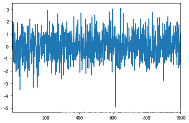
10.1.1 Series：

ts=pd.Series(np.random.randn(1000),index=list(range(1,1001)))
print(ts)

1       0.467369
2       0.657971
3       1.671581
4      -0.280581
5       1.662911
          ...   
996     0.167373
997    -1.364028
998    -0.269425
999     0.413813
1000    1.025991
Length: 1000, dtype: float64

正常图像：

ts.plot()
plt.show()

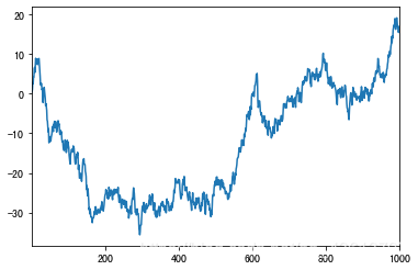
累计图像：

ts.cumsum().plot()
plt.show()

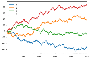
10.1.2 DataFrame：

df = pd.DataFrame(np.random.randn(1000,4),index=list(range(1,1001)),columns=['A','B','C','D'])
df  # print(df)

	A	B	C	D
1	0.876069	2.065587	-0.044876	-1.551308
2	-0.036537	-2.316728	-0.537699	0.168699
3	1.629338	-1.552489	-0.943307	0.657343
4	-0.214209	-0.538340	-0.399330	-0.726052
5	0.268486	-1.328338	-0.742542	0.223678
...	...	...	...	...
996	-0.644218	-0.081672	1.538658	-1.647879
997	-2.601843	-0.844147	0.085147	1.996194
998	-0.825643	0.330388	1.015113	1.195541
999	1.449490	0.966305	0.847445	-0.008207
1000	0.126165	0.882948	-0.168549	1.732745

1000 rows × 4 columns

正常图像：

df.plot()
plt.show()

累计图像：

df.cumsum().plot()
plt.show()

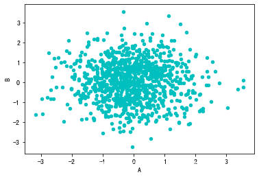
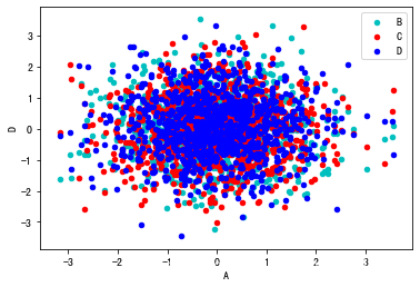
10.2 散点图(scatter)：

只能用于DataFrame

df.plot.scatter(x='A',y='B',color='c')
plt.show()

层叠显示：

pic1=df.plot.scatter(x='A',y='B',color='c',label='B')
pic2=df.plot.scatter(x='A', y='C', color='r', label='C', ax=pic1)
pic3=df.plot.scatter(x='A', y='D', color='b', label='D', ax=pic1)
plt.show()

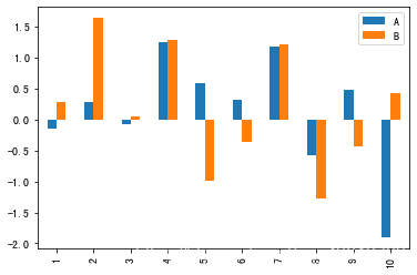
10.3 柱状图(bar/barh)：

df = pd.DataFrame(np.random.randn(10,2),index=list(range(1,11)),columns=['A','B'])
df # print(df)

	A	B
1	-0.145207	0.277669
2	0.284978	1.639432
3	-0.077486	0.056532
4	1.251053	1.289330
5	0.584433	-0.995018
6	0.325838	-0.370692
7	1.183686	1.217381
8	-0.581146	-1.273807
9	0.481801	-0.442896
10	-1.901283	0.424851

10.3.1 竖直柱状图：

df.plot.bar()
plt.show()

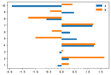
10.3.2 水平柱状图：

df.plot.barh()
plt.show()

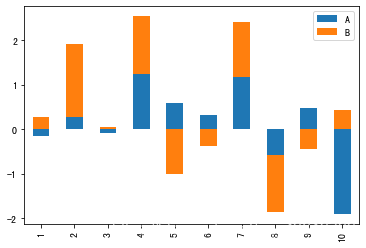
10.3.3 堆叠柱状图：

df.plot.bar(stacked=True)
plt.show()

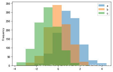
10.4 直方图(hist)：

df = pd.DataFrame({'a': np.random.randn(1000) + 1, 'b': np.random.randn(1000),'c': np.random.randn(1000) - 1}, columns=['a', 'b', 'c'])
df.plot.hist(alpha=0.5)
plt.show()

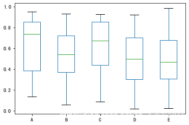
10.5 箱型图(box)：

df = pd.DataFrame(np.random.rand(10, 5), columns=['A', 'B', 'C', 'D', 'E'])
df.plot.box()
plt.show()

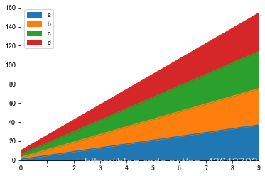
10.6 面积图(area)：

df = pd.DataFrame(np.arange(1,41).reshape(10,4), columns=['a', 'b', 'c', 'd'])
df.plot.area()
plt.show()

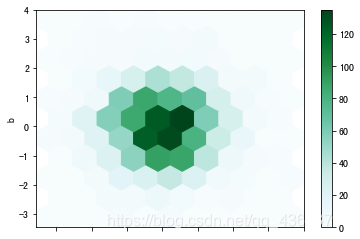
10.7 六角形箱体图(hexbin)：

df = pd.DataFrame(np.random.randn(2000, 2), columns=['a', 'b'])
df.plot.hexbin(x='a', y='b', gridsize=10)
plt.show()

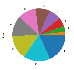
10.8 饼图(pie)：

10.8.1 Series：

ps=pd.Series([_ for _ in range(11)])
ps.plot.pie()
plt.show()

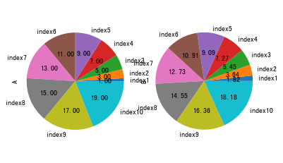
10.8.2 DataFrame：

df = pd.DataFrame(np.arange(1, 21).reshape(10, 2), index=["index{}".format(_)for _ in range(1, 11)], columns=['A', 'B'])
df.plot.pie(subplots=True,  autopct='%.2f', legend=False)
plt.axis('equal')
plt.show()

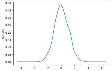
10.9 密度图(kde)：

ps = pd.Series(np.random.randn(1000))
ps.plot.kde()
plt.show()

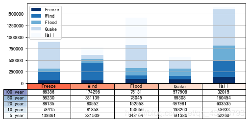
10.10 一个综合例子：

(来源网络,但是源头在哪里我也说不清…)

data = [[66386, 174296,  75131, 577908,  32015],
        [58230, 381139,  78045,  99308, 160454],
        [89135,  80552, 152558, 497981, 603535],
        [78415,  81858, 150656, 193263,  69638],
        [139361, 331509, 343164, 781380,  52269]]
columns = ('Freeze', 'Wind', 'Flood', 'Quake', 'Hail')
rows = ['%d year' % x for x in (100, 50, 20, 10, 5)]
df = pd.DataFrame(data, columns=('Freeze', 'Wind', 'Flood', 'Quake', 'Hail'),
                  index=['%d year' % x for x in (100, 50, 20, 10, 5)])
df.plot(kind='bar', grid=True, colormap='Blues_r',
        stacked=True, figsize=(8, 3))
plt.table(cellText=data,
          cellLoc='center',
          cellColours=None,
          rowLabels=rows,
          rowColours=plt.cm.BuPu(np.linspace(0, 0.5, 5))[::-1],
          colLabels=columns,
          colColours=plt.cm.Reds(np.linspace(0, 0.5, 5))[::-1],
          rowLoc='right',
          loc='bottom')
plt.xticks([])
plt.show()

11 数据获取与导出：

df = pd.DataFrame(data=np.random.randn(10, 10))
df  # print(df)

	0	1	2	3	4	5	6	7	8	9
0	1.068240	-1.151127	-0.754891	0.414021	0.638704	-0.020647	-0.448307	-0.382925	1.309449	-1.166587
1	-1.281921	2.132671	0.733787	-0.054124	-1.147173	-2.450771	-0.100820	0.848969	-0.107513	0.785965
2	0.408719	0.915703	-0.409178	-0.244410	-1.155077	-0.050631	0.376198	-0.535242	0.958951	0.263776
3	1.587115	-0.111936	-0.291101	-1.616078	-1.637145	0.520931	0.608293	1.659118	-1.352053	-0.742237
4	-0.416936	-1.201720	-0.536394	-2.332946	-1.145977	-0.361430	-0.173924	2.108183	1.225851	1.183785
5	-1.038260	0.601028	-1.109006	-1.528502	0.278005	0.476453	-0.232497	-1.680161	0.032745	0.518991
6	0.006007	0.756336	0.554774	-0.182611	0.117581	0.091906	-1.184422	0.621687	0.247616	-0.243130
7	-1.105260	0.602079	0.267793	-0.564271	-1.596596	-0.959563	-1.428516	0.000715	-0.769573	0.537807
8	-0.015989	0.331866	-0.106719	-0.359950	0.630097	0.598659	0.390666	-0.710734	0.861856	0.060555
9	0.615639	-1.112035	-0.003613	0.252591	-0.674543	-0.136806	1.322243	-0.029689	-0.746584	2.128872

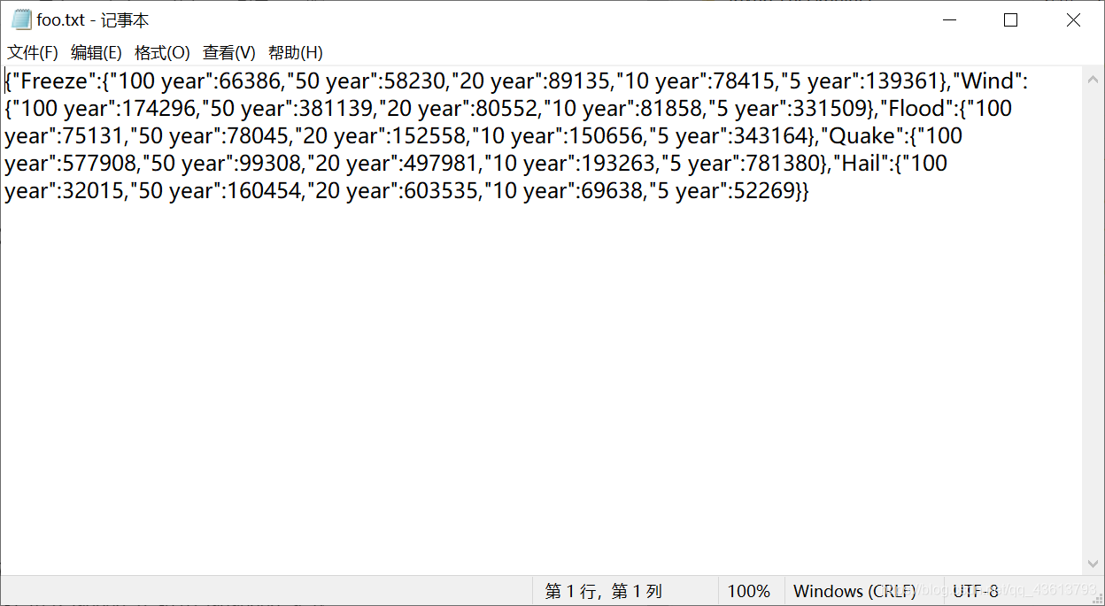
11.1 json：

11.1.1 保存为json格式：

dfj = df.to_json("foo.txt")

11.1.2 从json中读取数据：

pds = pd.read_json("foo.txt")
pds  # print(pds)

	0	1	2	3	4	5	6	7	8	9
0	1.068240	-1.151127	-0.754891	0.414021	0.638704	-0.020647	-0.448307	-0.382925	1.309449	-1.166587
1	-1.281921	2.132671	0.733787	-0.054124	-1.147173	-2.450771	-0.100820	0.848969	-0.107513	0.785965
2	0.408719	0.915703	-0.409178	-0.244410	-1.155077	-0.050631	0.376198	-0.535242	0.958951	0.263776
3	1.587115	-0.111936	-0.291101	-1.616078	-1.637145	0.520931	0.608293	1.659118	-1.352053	-0.742237
4	-0.416936	-1.201720	-0.536394	-2.332946	-1.145977	-0.361430	-0.173924	2.108183	1.225851	1.183785
5	-1.038260	0.601028	-1.109006	-1.528502	0.278005	0.476453	-0.232497	-1.680161	0.032745	0.518991
6	0.006007	0.756336	0.554774	-0.182611	0.117581	0.091906	-1.184422	0.621687	0.247616	-0.243130
7	-1.105260	0.602079	0.267793	-0.564271	-1.596596	-0.959563	-1.428516	0.000715	-0.769573	0.537807
8	-0.015989	0.331866	-0.106719	-0.359950	0.630097	0.598659	0.390666	-0.710734	0.861856	0.060555
9	0.615639	-1.112035	-0.003613	0.252591	-0.674543	-0.136806	1.322243	-0.029689	-0.746584	2.128872

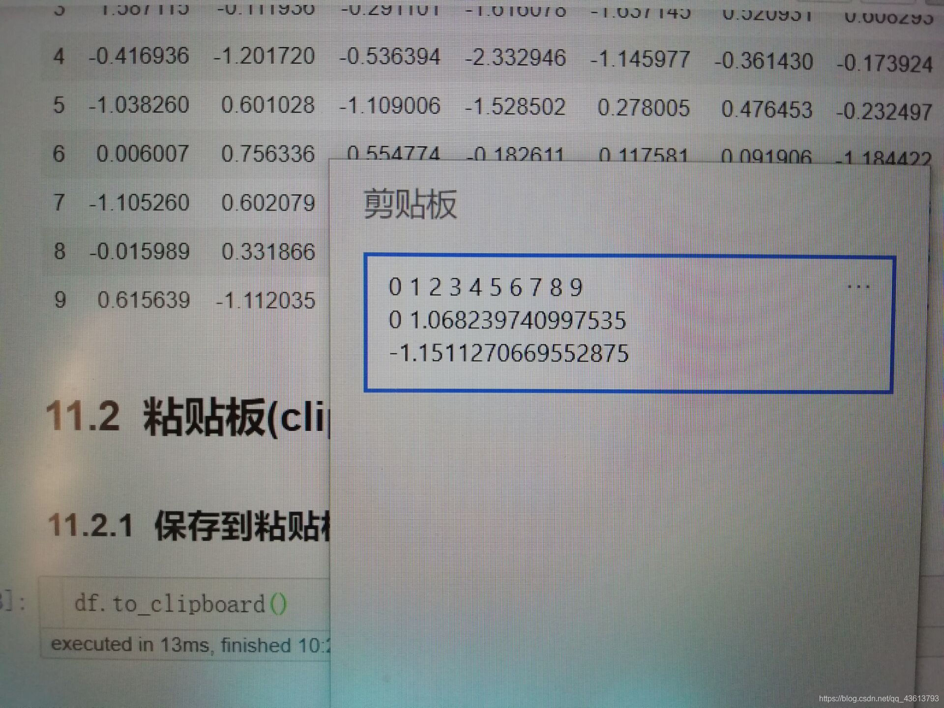
11.2 粘贴板(clipboard)：

11.2.1 保存到粘贴板：

df.to_clipboard()

（因为打开剪贴板的时候不能截屏，所以我就拍照了…）

11.2.2 从粘贴板中读取数据：

df1 = pd.read_clipboard()
df1  # print(df1)

	0	1	2	3	4	5	6	7	8	9
0	1.068240	-1.151127	-0.754891	0.414021	0.638704	-0.020647	-0.448307	-0.382925	1.309449	-1.166587
1	-1.281921	2.132671	0.733787	-0.054124	-1.147173	-2.450771	-0.100820	0.848969	-0.107513	0.785965
2	0.408719	0.915703	-0.409178	-0.244410	-1.155077	-0.050631	0.376198	-0.535242	0.958951	0.263776
3	1.587115	-0.111936	-0.291101	-1.616078	-1.637145	0.520931	0.608293	1.659118	-1.352053	-0.742237
4	-0.416936	-1.201720	-0.536394	-2.332946	-1.145977	-0.361430	-0.173924	2.108183	1.225851	1.183785
5	-1.038260	0.601028	-1.109006	-1.528502	0.278005	0.476453	-0.232497	-1.680161	0.032745	0.518991
6	0.006007	0.756336	0.554774	-0.182611	0.117581	0.091906	-1.184422	0.621687	0.247616	-0.243130
7	-1.105260	0.602079	0.267793	-0.564271	-1.596596	-0.959563	-1.428516	0.000715	-0.769573	0.537807
8	-0.015989	0.331866	-0.106719	-0.359950	0.630097	0.598659	0.390666	-0.710734	0.861856	0.060555
9	0.615639	-1.112035	-0.003613	0.252591	-0.674543	-0.136806	1.322243	-0.029689	-0.746584	2.128872

11.3 csv

11.3.1 保存到csv：

df.to_csv('foo.csv')

11.3.2 从csv中读取数据：

df = pd.read_csv('foo.csv')
df  # print(df)

	Unnamed: 0	0	1	2	3	4	5	6	7	8	9
0	0	1.068240	-1.151127	-0.754891	0.414021	0.638704	-0.020647	-0.448307	-0.382925	1.309449	-1.166587
1	1	-1.281921	2.132671	0.733787	-0.054124	-1.147173	-2.450771	-0.100820	0.848969	-0.107513	0.785965
2	2	0.408719	0.915703	-0.409178	-0.244410	-1.155077	-0.050631	0.376198	-0.535242	0.958951	0.263776
3	3	1.587115	-0.111936	-0.291101	-1.616078	-1.637145	0.520931	0.608293	1.659118	-1.352053	-0.742237
4	4	-0.416936	-1.201720	-0.536394	-2.332946	-1.145977	-0.361430	-0.173924	2.108183	1.225851	1.183785
5	5	-1.038260	0.601028	-1.109006	-1.528502	0.278005	0.476453	-0.232497	-1.680161	0.032745	0.518991
6	6	0.006007	0.756336	0.554774	-0.182611	0.117581	0.091906	-1.184422	0.621687	0.247616	-0.243130
7	7	-1.105260	0.602079	0.267793	-0.564271	-1.596596	-0.959563	-1.428516	0.000715	-0.769573	0.537807
8	8	-0.015989	0.331866	-0.106719	-0.359950	0.630097	0.598659	0.390666	-0.710734	0.861856	0.060555
9	9	0.615639	-1.112035	-0.003613	0.252591	-0.674543	-0.136806	1.322243	-0.029689	-0.746584	2.128872

11.4 HDF5：

生成HDF5存储（需要安装tables库 pip install tables）

11.4.1 保存到HDF5：

df.to_hdf('foo.h5','df')

11.4.2 从HDF5存储中读入数据：

df=pd.read_hdf('foo.h5','df')
df # print(df)

	Unnamed: 0	0	1	2	3	4	5	6	7	8	9
0	0	1.068240	-1.151127	-0.754891	0.414021	0.638704	-0.020647	-0.448307	-0.382925	1.309449	-1.166587
1	1	-1.281921	2.132671	0.733787	-0.054124	-1.147173	-2.450771	-0.100820	0.848969	-0.107513	0.785965
2	2	0.408719	0.915703	-0.409178	-0.244410	-1.155077	-0.050631	0.376198	-0.535242	0.958951	0.263776
3	3	1.587115	-0.111936	-0.291101	-1.616078	-1.637145	0.520931	0.608293	1.659118	-1.352053	-0.742237
4	4	-0.416936	-1.201720	-0.536394	-2.332946	-1.145977	-0.361430	-0.173924	2.108183	1.225851	1.183785
5	5	-1.038260	0.601028	-1.109006	-1.528502	0.278005	0.476453	-0.232497	-1.680161	0.032745	0.518991
6	6	0.006007	0.756336	0.554774	-0.182611	0.117581	0.091906	-1.184422	0.621687	0.247616	-0.243130
7	7	-1.105260	0.602079	0.267793	-0.564271	-1.596596	-0.959563	-1.428516	0.000715	-0.769573	0.537807
8	8	-0.015989	0.331866	-0.106719	-0.359950	0.630097	0.598659	0.390666	-0.710734	0.861856	0.060555
9	9	0.615639	-1.112035	-0.003613	0.252591	-0.674543	-0.136806	1.322243	-0.029689	-0.746584	2.128872

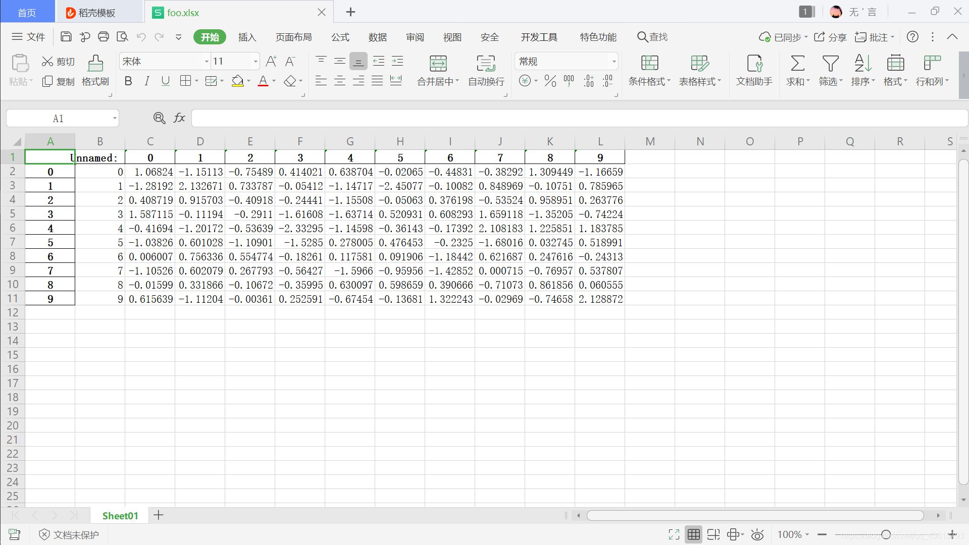
11.5 excel：

生成Excel文件（需要安装openpyxl库 pip install openpyxl）

11.5.1 保存到excel：

df.to_excel('foo.xlsx',sheet_name='Sheet01')

11.5.2 从excel中读取数据：

df=pd.read_excel('foo.xlsx', 'Sheet01',index_col=None, na_values=['NA'])
df # print(df)

	Unnamed: 0	Unnamed: 0.1	0	1	2	3	4	5	6	7	8	9
0	0	0	1.068240	-1.151127	-0.754891	0.414021	0.638704	-0.020647	-0.448307	-0.382925	1.309449	-1.166587
1	1	1	-1.281921	2.132671	0.733787	-0.054124	-1.147173	-2.450771	-0.100820	0.848969	-0.107513	0.785965
2	2	2	0.408719	0.915703	-0.409178	-0.244410	-1.155077	-0.050631	0.376198	-0.535242	0.958951	0.263776
3	3	3	1.587115	-0.111936	-0.291101	-1.616078	-1.637145	0.520931	0.608293	1.659118	-1.352053	-0.742237
4	4	4	-0.416936	-1.201720	-0.536394	-2.332946	-1.145977	-0.361430	-0.173924	2.108183	1.225851	1.183785
5	5	5	-1.038260	0.601028	-1.109006	-1.528502	0.278005	0.476453	-0.232497	-1.680161	0.032745	0.518991
6	6	6	0.006007	0.756336	0.554774	-0.182611	0.117581	0.091906	-1.184422	0.621687	0.247616	-0.243130
7	7	7	-1.105260	0.602079	0.267793	-0.564271	-1.596596	-0.959563	-1.428516	0.000715	-0.769573	0.537807
8	8	8	-0.015989	0.331866	-0.106719	-0.359950	0.630097	0.598659	0.390666	-0.710734	0.861856	0.060555
9	9	9	0.615639	-1.112035	-0.003613	0.252591	-0.674543	-0.136806	1.322243	-0.029689	-0.746584	2.128872

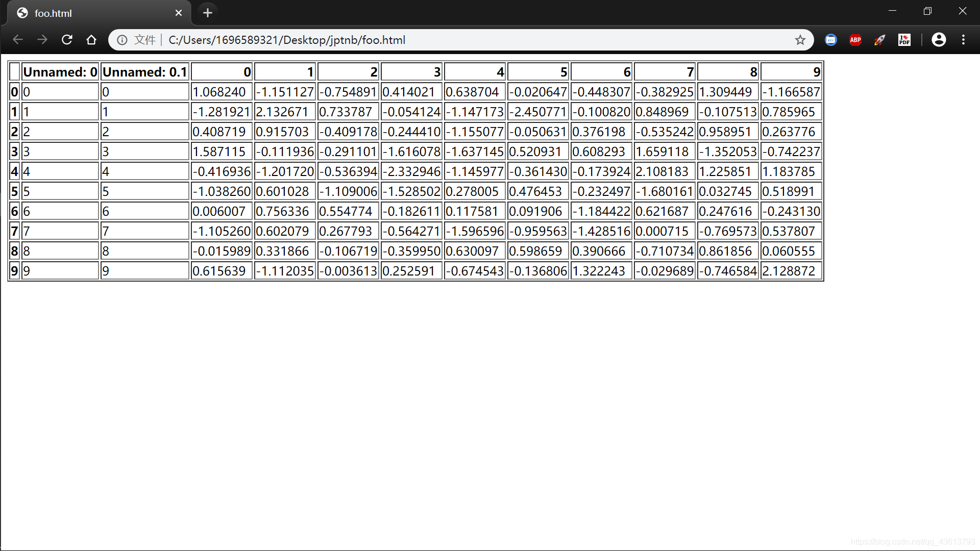
11.6 html：

11.6.1 保存到html：

df.to_html("foo.html")

11.6.2 从html中读取数据:

df1=pd.read_html('foo.html')
df1 # print(df)

[   Unnamed: 0  Unnamed: 0.1  Unnamed: 0.1.1         0         1         2  \
 0           0             0               0  1.068240 -1.151127 -0.754891   
 1           1             1               1 -1.281921  2.132671  0.733787   
 2           2             2               2  0.408719  0.915703 -0.409178   
 3           3             3               3  1.587115 -0.111936 -0.291101   
 4           4             4               4 -0.416936 -1.201720 -0.536394   
 5           5             5               5 -1.038260  0.601028 -1.109006   
 6           6             6               6  0.006007  0.756336  0.554774   
 7           7             7               7 -1.105260  0.602079  0.267793   
 8           8             8               8 -0.015989  0.331866 -0.106719   
 9           9             9               9  0.615639 -1.112035 -0.003613   
 
           3         4         5         6         7         8         9  
 0  0.414021  0.638704 -0.020647 -0.448307 -0.382925  1.309449 -1.166587  
 1 -0.054124 -1.147173 -2.450771 -0.100820  0.848969 -0.107513  0.785965  
 2 -0.244410 -1.155077 -0.050631  0.376198 -0.535242  0.958951  0.263776  
 3 -1.616078 -1.637145  0.520931  0.608293  1.659118 -1.352053 -0.742237  
 4 -2.332946 -1.145977 -0.361430 -0.173924  2.108183  1.225851  1.183785  
 5 -1.528502  0.278005  0.476453 -0.232497 -1.680161  0.032745  0.518991  
 6 -0.182611  0.117581  0.091906 -1.184422  0.621687  0.247616 -0.243130  
 7 -0.564271 -1.596596 -0.959563 -1.428516  0.000715 -0.769573  0.537807  
 8 -0.359950  0.630097  0.598659  0.390666 -0.710734  0.861856  0.060555  
 9  0.252591 -0.674543 -0.136806  1.322243 -0.029689 -0.746584  2.128872  ]