基于已有的信息预测当遇难时,是否可以获救
第一步,提取出最有价值的信息
survived→0表示遇难,1表示幸存
Pclass→舱室类型
Name→遇难者姓名
Sex→性别
Age→年龄
SibSp→有多少亲人一起来坐船
Parch→身边有多少老人和孩子
Ticket→票的编号
Fare→票价
Cabin→舱号
Eabarked→在不同的站区上的车
第二步,制作出分类器完成预测是否可以获救
(一)导入数据
import pandas
titanic = pandas.read_csv("titanic_train.csv")    #导入数据
titanic.head(5)    #打印出前5行数据观察

(二)缺失值的填充
titanic["Age"] = titanic["Age"].fillna(titanic["Age"].median())   #用均值对“Age”特征的缺失值进行填充
print titanic.describe()      #打印出各特征的属性

(三)对于字符量将其映射成数值的量
①转换“Sex”列
print titanic["Sex"].unique()    #打印出“Sex”特征组中的所有可能性

titanic.loc[titanic["Sex"] == "male", "Sex"] = 0
titanic.loc[titanic["Sex"] == "female", "Sex"] = 1
输出[‘male’ ‘female’]
②转换“Eabrked”列
print titanic["Embarked"].unique()
titanic["Embarked"] = titanic["Embarked"].fillna('S')   #对非连续的值进行填充,谁多用谁填充
titanic.loc[titanic["Embarked"] == "S", "Embarked"] = 0
titanic.loc[titanic["Embarked"] == "C", "Embarked"] = 1
titanic.loc[titanic["Embarked"] == "Q", "Embarked"] = 2
输出[‘S’ ‘C’ ‘Q’ nan]
nan表示的有缺失值
观察数据,谁最多用谁填充
(四)应用机器学习算法来实现分类
Ⅰ在训练集中预处理与操作
①通过线性回归
#导入线性回归
from sklearn.linear_model import LinearRegression
#Sklearn还具有一个帮助程序,可以轻松进行交叉验证
from sklearn.cross_validation import KFold

#我们用来预测目标的列(特征)
predictors = ["Pclass", "Sex", "Age", "SibSp", "Parch", "Fare", "Embarked"]

#初始化我们的算法类
alg = LinearRegression()

#为泰坦尼克号数据集生成交叉验证折叠。它返回与训练和测试对应的行索引。
#我们设置随机状态以确保每次运行此操作时得到相同的拆分。
kf = KFold(titanic.shape[0], n_folds=3, random_state=1)

predictions = []
for train, test in kf:
    # 我们正在使用的预测变量训练算法。 注意我们如何在训练集中取行。
    train_predictors = (titanic[predictors].iloc[train,:])    #把train的数据拿到手

    #我们用来训练算法的目标。
    train_target = titanic["Survived"].iloc[train]    #把训练的标签拿到手

    # 利用预测器和目标对算法进行训练。
    alg.fit(train_predictors, train_target)

    #我们现在可以在测试中做出预测了
    test_predictions = alg.predict(titanic[predictors].iloc[test,:])
    predictions.append(test_predictions)
通过线性回归得到的结果进行比较,若<0.5未获救,>.5的则获救
import numpy as np

#这些预测是在三个独立的numpy数组中进行的。将它们连接成一个。
#我们将它们连接在轴0上,因为它们只有一个轴。
predictions = np.concatenate(predictions, axis=0)

#将预测映射到结果(只有可能的结果是1和0)
predictions[predictions > .5] = 1
predictions[predictions <=.5] = 0
accuracy = sum(predictions[predictions == titanic["Survived"]]) / len(predictions)   #预测的和真实给定的label进行比较
print accuracy    #打印出准确率
输出 0.783389450056
②通过逻辑回归
from sklearn import cross_validation
from sklearn.linear_model import LogisticRegression

#初始化我们的算法
alg = LogisticRegression(random_state=1)

#计算所有交叉验证折叠的准确度得分。(比以前简单多了!)
scores = cross_validation.cross_val_score(alg, titanic[predictors], titanic["Survived"], cv=3)

#取分数的平均数(因为我们每叠有一个)
print(scores.mean())
输出 0.787878787879
Ⅱ在测试集中进行预处理与操作
titanic_test = pandas.read_csv("test.csv")
titanic_test["Age"] = titanic_test["Age"].fillna(titanic["Age"].median())
titanic_test["Fare"] = titanic_test["Fare"].fillna(titanic_test["Fare"].median())
titanic_test.loc[titanic_test["Sex"] == "male", "Sex"] = 0
titanic_test.loc[titanic_test["Sex"] == "female", "Sex"] = 1
titanic_test["Embarked"] = titanic_test["Embarked"].fillna("S")

titanic_test.loc[titanic_test["Embarked"] == "S", "Embarked"] = 0
titanic_test.loc[titanic_test["Embarked"] == "C", "Embarked"] = 1
titanic_test.loc[titanic_test["Embarked"] == "Q", "Embarked"] = 2
(五)使用随机森林分类器改进模型
①建立随机森林模型
from sklearn import cross_validation
from sklearn.ensemble import RandomForestClassifier

predictors = ["Pclass", "Sex", "Age", "SibSp", "Parch", "Fare", "Embarked"]

#用默认参数初始化我们的算法
#n_estimators 是我们要造的树的数目
#min_samples_split 是进行拆分所需的最小行数
#min_samples_leaf 是在树枝结束的地方(树的底部)我们可以拥有的最小样本数。
alg = RandomForestClassifier(random_state=1, n_estimators=10, min_samples_split=2, min_samples_leaf=1)

#计算所有交叉验证折叠的准确度得分。(比以前简单多了!)
kf = cross_validation.KFold(titanic.shape[0], n_folds=3, random_state=1)
scores = cross_validation.cross_val_score(alg, titanic[predictors], titanic["Survived"], cv=kf)

#取分数的平均数(因为我们每叠有一个)
print(scores.mean())
输出为 0.785634118967
②发现其输出与回归模型相似,调整随机森林的参数(很花时间)
alg = RandomForestClassifier(random_state=1, n_estimators=100, min_samples_split=4, min_samples_leaf=2)

#计算所有交叉验证折叠的准确度得分。(比以前简单多了!)
kf = cross_validation.KFold(titanic.shape[0], 3, random_state=1)
scores = cross_validation.cross_val_score(alg, titanic[predictors], titanic["Survived"], cv=kf)

#取分数的平均数(因为我们每叠有一个)
print(scores.mean())
输出 0.814814814815
③难以通过参数选择提升精度时,额外再提取一些特征让分类器去学习(增加一些新的特征)
#生成一个新的"familysize"特征,把所有家庭成员加到一起,有可能家庭成员的数量对逃生有一定影响
titanic["FamilySize"] = titanic["SibSp"] + titanic["Parch"]

#假设名字的长度和获救有关
titanic["NameLength"] = titanic["Name"].apply(lambda x: len(x))
#提取名字的称谓特征,假设称谓的不同对是否获救也有关联
import re
#从名称中获取标题的函数。
def get_title(name):
#使用正则表达式搜索标题。标题总是由大写和小写字母组成,并以句号结尾。
title_search = re.search(' ([A-Za-z]+)\.', name)
#如果标题存在,则提取并返回它。
if title_search:
return title_search.group(1)
return " "
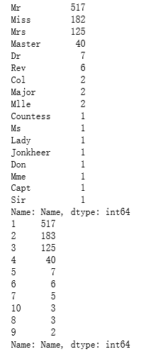
#获取所有标题并打印每个标题出现的频率。
titles = titanic["Name"].apply(get_title)
print(pandas.value_counts(titles))
#将每个标题映射为整数。有些标题非常罕见,并且被压缩成与其他标题相同的代码。
title_mapping = {"Mr": 1, "Miss": 2, "Mrs": 3, "Master": 4, "Dr": 5, "Rev": 6, "Major": 7, "Col": 7, "Mlle": 8, "Mme": 8, "Don": 9, "Lady": 10, "Countess": 10, "Jonkheer": 10, "Sir": 9, "Capt": 7, "Ms": 2}
for k,v in title_mapping.items():
titles[titles == k] = v
#确认我们转换了所有内容。
print(pandas.value_counts(titles))
#在“标题”列中添加。
titanic["Title"] = titles
④增加了一部分后,对这些特征进行衡量选出最有价值的特征
验证方法:建立随机森林模型后会得到一个错误率erroB1,若想知道其中一个特征有多大的重要性,把这个特征的列完全破坏掉后得到的错误率erroB2,观察这两次准确率的差值,若相差不多,则说明这一列特征不重要
用feature_selection这个库,选择哪个特征是最重要的
import numpy as np
from sklearn.feature_selection import SelectKBest, f_classif
import matplotlib.pyplot as plt
predictors = ["Pclass", "Sex", "Age", "SibSp", "Parch", "Fare", "Embarked", "FamilySize", "Title", "NameLength"]      #候选特征

#对特征进行选择
selector = SelectKBest(f_classif, k=5)
selector.fit(titanic[predictors], titanic["Survived"])   #通过“Survived”这个Label去衡量每一个特征的重要性

#之后两部分就是画图流程
#获取每个特征的原始p值,并从p值转换为分数
scores = -np.log10(selector.pvalues_)

#画出分数。看看“阶级”、“性别”、“头衔”和“费用”哪一个最好的?
plt.bar(range(len(predictors)), scores)
plt.xticks(range(len(predictors)), predictors, rotation='vertical')
plt.show()

#只选择四个最好的特征。
predictors = ["Pclass", "Sex", "Fare", "Title"]

alg = RandomForestClassifier(random_state=1, n_estimators=50, min_samples_split=8, min_samples_leaf=4)
**从图中可以剔除对是否获救影响不重要的特征

(六)用集成的方法来做
from sklearn.ensemble import GradientBoostingClassifier
import numpy as np

#我们要集成的算法。
#我们对logistic回归使用了更多的线性预测,所有的都使用了梯度增强分类器。
algorithms = [
    [GradientBoostingClassifier(random_state=1, n_estimators=25, max_depth=3), ["Pclass", "Sex", "Age", "Fare", "Embarked", "FamilySize", "Title",]],
    [LogisticRegression(random_state=1), ["Pclass", "Sex", "Fare", "FamilySize", "Title", "Age", "Embarked"]]
]           #将两个算法集成在一起


#初始化交叉验证折叠
kf = KFold(titanic.shape[0], n_folds=3, random_state=1)

predictions = []
for train, test in kf:
    train_target = titanic["Survived"].iloc[train]
    full_test_predictions = []
    #对每个折叠上的每个算法进行预测
    for alg, predictors in algorithms:
        #在训练数据上拟合算法。

        alg.fit(titanic[predictors].iloc[train,:], train_target)
        #选择并预测测试折叠。
        #.astype(float)是将数据帧转换为所有float并避免sklearn错误所必需的。
        test_predictions = alg.predict_proba(titanic[predictors].iloc[test,:].astype(float))[:,1]
        full_test_predictions.append(test_predictions)

    #使用一个简单的加密方案——只需平均预测就可以得到最终的分类。
    test_predictions = (full_test_predictions[0] + full_test_predictions[1]) / 2   #把两次预测的结果加在一起除二求平均值
    #任何大于.5的值都假定为1预测,小于.5的值则为0预测。
    test_predictions[test_predictions <= .5] = 0
    test_predictions[test_predictions > .5] = 1
    predictions.append(test_predictions)

#把所有的预测放在一个数组中。
predictions = np.concatenate(predictions, axis=0)

#通过与训练数据的比较计算精度。
accuracy = sum(predictions[predictions == titanic["Survived"]]) / len(predictions)
print(accuracy)
输出 0.821548821549
titles = titanic_test["Name"].apply(get_title)
#我们在图上添加了dona标题,因为它在测试集中,而不是训练集中
title_mapping = {"Mr": 1, "Miss": 2, "Mrs": 3, "Master": 4, "Dr": 5, "Rev": 6, "Major": 7, "Col": 7, "Mlle": 8, "Mme": 8, "Don": 9, "Lady": 10, "Countess": 10, "Jonkheer": 10, "Sir": 9, "Capt": 7, "Ms": 2, "Dona": 10}
for k,v in title_mapping.items():
titles[titles == k] = v
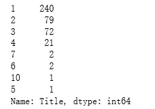
titanic_test["Title"] = titles
#检查每个唯一标题的计数。
print(pandas.value_counts(titanic_test["Title"]))
#现在,我们添加“FamilySize”列。
titanic_test["FamilySize"] = titanic_test["SibSp"] + titanic_test["Parch"]
predictors = ["Pclass", "Sex", "Age", "Fare", "Embarked", "FamilySize", "Title"]

algorithms = [
    [GradientBoostingClassifier(random_state=1, n_estimators=25, max_depth=3), predictors],
    [LogisticRegression(random_state=1), ["Pclass", "Sex", "Fare", "FamilySize", "Title", "Age", "Embarked"]]
]

full_predictions = []
for alg, predictors in algorithms:
    #使用完整的训练数据拟合算法。
    alg.fit(titanic[predictors], titanic["Survived"])
    #使用测试数据集进行预测。 我们必须将所有列都转换为浮点数以避免错误。
    predictions = alg.predict_proba(titanic_test[predictors].astype(float))[:,1]
    full_predictions.append(predictions)

#梯度提升分类器产生更好的预测,因此我们对其加权更高。
predictions = (full_predictions[0] * 3 + full_predictions[1]) / 4
predictions
输出
array([ 0.11682912,  0.47835566,  0.12614824,  0.13098157,  0.52105874,
        0.1435209 ,  0.64085331,  0.18003152,  0.67801353,  0.12111118,
        0.12105181,  0.20902118,  0.91068381,  0.1089127 ,  0.89142102,
        0.87713474,  0.16349859,  0.13907791,  0.54103238,  0.55661006,
        0.22420875,  0.5372079 ,  0.90572223,  0.38890588,  0.88384752,
        0.10357315,  0.90909441,  0.13746454,  0.31046249,  0.12665718,
        0.11663767,  0.18274855,  0.55220994,  0.49648575,  0.42415297,
        0.14191051,  0.50973638,  0.52452209,  0.13270506,  0.28366691,
        0.11145281,  0.46618807,  0.09996501,  0.83420617,  0.89959119,
        0.14983417,  0.31593419,  0.13789623,  0.89104185,  0.54189565,
        0.35666363,  0.17718135,  0.8307195 ,  0.87995521,  0.1755907 ,
        0.13741805,  0.10667279,  0.1234385 ,  0.12099736,  0.91285169,
        0.13099159,  0.15341948,  0.12993967,  0.66573206,  0.66343836,
        0.87272604,  0.67238712,  0.288265  ,  0.35236574,  0.85565507,
        0.6622414 ,  0.12701993,  0.55390065,  0.36740462,  0.91110312,
        0.41201902,  0.13014004,  0.83671279,  0.15614414,  0.6622414 ,
        0.68129213,  0.20605719,  0.20382623,  0.12105181,  0.18486634,
        0.13130212,  0.65680539,  0.53029858,  0.65489631,  0.79881212,
        0.53764546,  0.12104028,  0.8913725 ,  0.13014004,  0.28406245,
        0.12345367,  0.86792484,  0.14666337,  0.58599461,  0.12260781,
        0.90433464,  0.14730817,  0.13789623,  0.12262433,  0.62257491,
        0.13155874,  0.14607753,  0.13789623,  0.13020336,  0.17473033,
        0.14286392,  0.65490316,  0.89528117,  0.67146758,  0.88346017,
        0.13992078,  0.11805064,  0.69612515,  0.36668939,  0.86241698,
        0.87649291,  0.12609327,  0.90276371,  0.12099027,  0.13789623,
        0.56971935,  0.12608181,  0.63733743,  0.13339996,  0.13340574,
        0.12723637,  0.51609607,  0.23921874,  0.10791695,  0.09896737,
        0.12431124,  0.13346495,  0.16214099,  0.52029433,  0.12232635,
        0.20712059,  0.90529649,  0.19747926,  0.16153716,  0.42927593,
        0.10487176,  0.33642492,  0.13518414,  0.46618807,  0.34478758,
        0.91431377,  0.13214999,  0.10690998,  0.48983645,  0.11274825,
        0.12427868,  0.9107016 ,  0.57991631,  0.42927593,  0.51274048,
        0.65489239,  0.57884522,  0.82113381,  0.12096648,  0.28979611,
        0.58587108,  0.30130471,  0.14606803,  0.9025041 ,  0.52257377,
        0.12101884,  0.13299498,  0.12418534,  0.13207486,  0.1319655 ,
        0.8729358 ,  0.87633414,  0.29670328,  0.83389526,  0.85558679,
        0.15614414,  0.33352246,  0.90219082,  0.13789623,  0.91718918,
        0.13603003,  0.85482389,  0.12241402,  0.14217314,  0.13560687,
        0.1348803 ,  0.25547183,  0.49950989,  0.12729496,  0.71980831,
        0.10795469,  0.85516508,  0.58990449,  0.16645668,  0.53980354,
        0.64867969,  0.66329187,  0.60981573,  0.87333314,  0.16322638,
        0.25696649,  0.63083524,  0.16482591,  0.88984707,  0.12346408,
        0.12849653,  0.12097124,  0.24675029,  0.80199995,  0.41248342,
        0.29768148,  0.65492663,  0.21860346,  0.90027407,  0.13014004,
        0.8137002 ,  0.13611142,  0.84275393,  0.12700828,  0.87789288,
        0.59807994,  0.12518087,  0.65489631,  0.11487493,  0.1441311 ,
        0.25075165,  0.89266286,  0.11622683,  0.1379133 ,  0.34224639,
        0.12796773,  0.19365861,  0.14018901,  0.80948189,  0.89790832,
        0.87598967,  0.82598174,  0.33036559,  0.12105101,  0.33258156,
        0.28710745,  0.8790295 ,  0.16058987,  0.86241698,  0.59133092,
        0.74586492,  0.15434326,  0.39647431,  0.13354268,  0.12701864,
        0.12101884,  0.13789623,  0.13014004,  0.83005787,  0.12700585,
        0.10894954,  0.12701508,  0.85003763,  0.64929875,  0.16619539,
        0.12105181,  0.21821016,  0.12101884,  0.50973638,  0.14016481,
        0.34495861,  0.13789623,  0.91564   ,  0.6332826 ,  0.13207439,
        0.85713531,  0.15861636,  0.12500116,  0.14267175,  0.16811853,
        0.52045075,  0.66231856,  0.65489631,  0.64136782,  0.71198852,
        0.10601085,  0.12099027,  0.3627808 ,  0.13207486,  0.13014004,
        0.33304456,  0.59319589,  0.13207486,  0.50584352,  0.12081676,
        0.12263655,  0.77903176,  0.12665718,  0.33024483,  0.12028976,
        0.11813957,  0.17547887,  0.1216941 ,  0.13347145,  0.65489631,
        0.82133626,  0.33497525,  0.67696014,  0.20916505,  0.42575111,
        0.13912869,  0.13799529,  0.12102122,  0.61904744,  0.90111957,
        0.67393647,  0.23919457,  0.17328806,  0.12182854,  0.18522951,
        0.12262433,  0.13491478,  0.16214099,  0.45541306,  0.90601333,
        0.12509883,  0.86563776,  0.34598576,  0.14469719,  0.17034218,
        0.82147627,  0.32823572,  0.13207439,  0.64322911,  0.12183262,
        0.25111398,  0.15333425,  0.09370087,  0.20950803,  0.35411806,
        0.17507148,  0.118123  ,  0.1469565 ,  0.91556464,  0.33657652,
        0.618368  ,  0.16214099,  0.62462682,  0.1654289 ,  0.85157883,
        0.89603825,  0.16322638,  0.24472808,  0.16066609,  0.70031025,
        0.15642457,  0.85672648,  0.12105022,  0.13789623,  0.57255235,
        0.10418822,  0.87672475,  0.86918839,  0.13098157,  0.91914163,
        0.15715004,  0.1313025 ,  0.53322127,  0.89562968,  0.17356053,
        0.15319843,  0.90891499,  0.16307942,  0.13130575,  0.87654859,
        0.90969185,  0.48853359,  0.17002326,  0.19866966,  0.13510974,
        0.13789623,  0.14010265,  0.54133852,  0.5949924 ,  0.15905635,
        0.83276875,  0.12430276,  0.12019388,  0.14606637,  0.18789784,
        0.38579307,  0.87750065,  0.56459193,  0.12807839,  0.10318132,
        0.91169572,  0.14231524,  0.88773179,  0.12607946,  0.12971145,
        0.90753797,  0.12635163,  0.90891637,  0.35988713,  0.30442425,
        0.18966803,  0.1501521 ,  0.26822399,  0.65488945,  0.64585313,
        0.65489631,  0.90711865,  0.56933478,  0.13014004,  0.86010063,
        0.10126674,  0.13014004,  0.41850311])
总结
第一步:分析数据,提取出有用的特征
第二步:有缺失值时,视情况对缺失值进行补充
第三步:数值转量换,将字符量转换成数值
第四步:构建分类器
①先构建简单的回归模型,发现回归模型的效果不理想
②用RandomForest对模型检测率进行改进
③把特征做一个组合,观察出每个特征的重要性,选择重要的留下
④集成多个分类器来进行构建
