粗糙集 rough set theory

最近看到一篇文章上有用到关于粗糙集的理论，所以到网上查了些资料学习了一下，目前应该脑子里有一个大致的概念了，知道这是干啥的，能够用来做些什么工作。接下来就记录下对我理解这个概念很有帮助的一些资料以及我自己的一些理解，然后把我看到的那篇论文上的关于粗糙集的case也写一下。
————————————————————————————————————

对我理解粗糙集很有帮助的一些资料

1. 王国胤, 姚一豫, 于洪. 粗糙集理论与应用研究综述[J]. 计算机学报, 2009, 32(7).
   上述论文获取
2. 关于粗糙集一些概念通俗易懂的解释
3. 大佬写的博文，不过都是英文的
4. 维基百科，可以直接访问
5. 百度百科中的找到好工作的例子可以一看
6. 顺带看一眼好了

可以先看一下第一篇paper，对粗糙集的一些基本概念和拓展、运用有一个大致的理解，当然里面的概念都偏数学，比较难理解，所以不必全部都完全领会，先过一遍大致理解，心里有个印象，然后看一下第二篇文章，很通俗易懂，并且给了一个实际的例子，基本可以对粗糙集的概念进行理解了，第三篇是一个大佬记录的wiki的关于粗糙集的内容，全是英文的，直接看有点累，不过看完前两个再看就轻松多了，第四个链接是维基百科，可以直接访问的，第五个和第六个也可以顺带一看，不看也OK。

《张文修, 吴伟志, 粱吉业, 李德玉. 粗糙集理论与方法[M]. 北京: 科学出版社,2001.》
《粗糙集理论、算法与应用》清华出版社
网上说上面两本书比较好，如果是要认真啃这块理论的话还是要看一看书的，当然我没看过拉，又一次感觉自己水水的。
——————————————————————————

我对粗糙集的理解

首先，先讲一下粗糙集中的一些最基本的概念，这些是对大致理解粗糙集必须的。

• 信息表
  下面这个例子就是一个信息表，来源于上面链接中的论文。

个体编号	头疼	肌肉疼	体温	流感
x1	是	是	正常	否
x2	是	是	高	是
x3	是	是	很高	是
x4	否	是	正常	否
x5	否	否	高	否
x6	否	是	很高	是

信息表 M 可以形式化地表达为四元组 $M =(U , A_t , {V_a|a ∈ A_t}, {I_a| a ∈ A_t})$ 表 1 中, U ={x1 , x2 , …, x6}是有限非空对象的集合,也称为论域，A_t ={头疼 ,肌肉疼, 体温, 流感}是有限非空的属性集合。 $V_a$ 表示属性 $a ∈ A_t$ 的属性值的范围 ,即属性 a的值域, $I_a :U -> V_a$是一个信息函数 .如果 $A\subseteq A_t$ , 则 $I_A(x)$表示 U 中对象 x 在属性 A 上的属性值。

• 概念、内涵（公式）、外延
  信息表 M 中的概念就是 $( \phi , m(\phi))$。概念 $( \phi, m(\phi))$的内涵是 $\phi$ , 表示 M 中对对象子集 $m(\phi)$的描述;概念 $( \phi, m(\phi))$的外延是 $m(\phi)$, 其含义是满足公式 $\phi$的所有对象的全体 。
  其中的 $\phi$就是公式，也是概念的内涵，举个例子的话就是（头疼=是）U （肌肉疼=否），可以是各个属性的公式的并。外延的话也就是这个公式所确定的子集。一个公式也可以确定一个划分，即通过某个公式可以将论域中所有的object进行划分。

• 条件属性、决策属性
  条件属性就是用来划分信息表的属性，决策属性就是需要利用条件属性进行判断的属性。在上述的信息表中，决策属性是“流感”，其余都是条件属性。

• 可定义集、语言
  我们用符号 (A)表示由属性子集 A定义的语言。
  在信息表 M 中, 如果称子集 $X \subseteq U$是可被属性子集 $A \subseteq A_t$ 定义的 , 当且仅当在语言(A)中存在一个公式 使得 $X =m(\phi)$.否则 , X 称为不可定义的。
  我们考虑属性子集 A ={头疼, 肌肉疼},语言（A）我的理解就是一个公式的集合，里面包含了所有可能的公式，对于上述的信息表，语言(A)就是 { (头疼=是) , （头疼=否） ， （肌肉疼=是） ，（肌肉疼=否）}.
  于是可定义集的全体表示为 $Def(U , (A))={m(\phi) | \phi∈(A)}$如果概念的外延能用逻辑公式简洁地表达 , 那它就是一个可定义的概念;从这个角度讲 ,概念的外延就是可定义集。

• 等价类
  如果两个对象 $x _i , x_j$是等价的 ,那么他们在语言 (A)中由相同的公式描述, 或者说他们在A 上的各个属性值相同。刚才得到的可定义集就是属性集合 A 上的等价关系 E(A)在论域U 上产生的划分,记为 $U/E(A)={[ x]_{E(A)} | x ∈ U}$, $[ x]_{E(A)}$是由关系 E(A)确定的等价类, 同一个等价类中的对象是不可分辨的，所以，有时我们也称等价关系为不可分辨关系。上例中，我们考虑属性子集 A ={头疼, 肌肉疼}， $U/E (A)=\{ \{x_1 , x_2 , x_3 \} , \{x_4 , x_6\} , \{x_5\}\}$。
  E(A)的等价类其实就是通过属性A对论域进行一个划分。可定义集就是E(A)的等价类或其某几个划分的并集。

• 上下近似
  这个是重点，也就是通过这个概念引出了粗糙集。
  针对不可定义集, 显然不可能构造一个公式来精确描述,只能通过上下界逼近的方式来刻画, 这就是粗糙集理论中的上下近似算子。设 E(A)是信息表 M 上的等价关系, $X\subseteq U$ , 上下近似算子 $\overline{apr(X)}$, $\underline{apr(X)}$(下文我们采用缩写形式 $\overline{apr(X)}$ , $\underline{apr(X)}$)定义为：
  $\overline{apr(X)}=∪\{Y|Y ∈ σ(U/E(A)), Y ∩ X ≠ \emptyset \} =∩\{Y | Y ∈ Def(U , (A), X \subseteq Y\}$
  $\underline{apr(X)}=∪\{Y|Y ∈ σ(U/E(A)), Y \subseteq X \} =∩\{Y | Y ∈ Def(U , (A), Y \subseteq X\}$
  上近似 $\overline{apr(X)}$是包含 X 的最小可定义集 , 下近似 $\underline{apr(X)}$是包含在 X 中的最大可定义集 .
  根据定义 , 可定义集显然有相同的上下近似。刚才我们在可定义的基础上构造了一对近似算子。也就是说 ,只有当对象不可定义时 ,才会用上下近似的方法来描述。
  下近似的计算方法： lower approximation is the union of all equivalence classes in $[x]_P$ which are contained by (i.e., are subsets of) the target set.
  上近似的计算方法： upper approximation is the union of all equivalence classes in $[x]_P$ which have non-empty intersection with the target set.

• 正负域
  考虑子集 $X\subseteq U$ ,论域空间将被分成 3 个区域 :
  (1)集合 X 的正域 :
  $POS(X)=\underline{apr(X)}$
  (2)集合 X 的负域 :
  $NEG(X)=POS(～ X)=U - \overline{apr(X)}$
  (3)集合 X 的边界域:
  $BND(X)=\overline{apr(X)}-\underline{apr(X)}$
  如果 BND(X)是空集, 则称集合 X 关于关系E(A)是清晰的(crisp);反之,如果 BND(X)不是空集,则称集合 X 为关于关系 E(A)粗糙的(rough).

• 粗糙集
  Pawlak定义由等价关系确定的等价类 $[x]_{E(A)}$的集合就组成了 P1-粗糙集集合(P1-Rough Set , PRS1).显然 , P1-粗糙集集合是子集集合, 即 $PRS1 =\{ [x]_{E(A)} | X \subseteq 2^U \}$.也可以给出和PRS1等价的关于粗糙集的另外一种定义 ,称为 P2-粗糙集集合.即 $PRS2 =\{<X 1 , X2>\}=\{〈{\underline{apr(X)}}, {\overline {apr(X)}}〉\}$.PRS1 和 PRS2 通称为 Pawlak 粗糙集.
  The tuple $\langle{\underline {apr(X)}},{\overline {apr(X)}}\rangle$ composed of the lower and upper approximation is called a rough set; thus, a rough set is composed of two crisp sets, one representing a lower boundary of the target set X, and the other representing an upper boundary of the target set X.

• 粗糙集准确性
  The accuracy of the rough-set representation of the set X : $\alpha_P(X)= \frac{ |{\underline{apr(X)}}| }{|{\overline{apr(X)}}| }$ That is, the accuracy of the rough set representation of $X, \alpha_{P}(X), 0 \leq \alpha_{P}(X) \leq 1$, is the ratio of the number of objects which can positively be placed in X to the number of objects that can possibly be placed in X. this provides a measure of how closely the rough set is approximating the target set.

• Reduct and core
  这个也就是属性简约了，找到对于某个决策属性而言最小的不可进一步缺少的条件属性集。
  Formally, a reduct is a subset of attributes $\mathrm{RED} \subseteq P$such that:

• $[x]_{\mathrm{RED}} = [x]_P$, that is, the equivalence classes induced by the reduced attribute set $\mathrm{RED}$ are the same as the equivalence class structure induced by the full attribute set P.

• the attribute set $\mathrm{RED}$ is minimal, in the sense that $[x]_{(\mathrm{RED}-\{a\})} \neq [x]_P$ for any attribute $a \in \mathrm{RED}$; in other words, no attribute can be removed from set $\mathrm{RED}$ without changing the equivalence classes $[x]_P$.

• Attribute dependency
  in rough set theory, the notion of dependency is defined very simply. Let us take two (disjoint) sets of attributes, set P and set Q, and inquire what degree of dependency obtains between them. Each attribute set induces an (indiscernibility) equivalence class structure, the equivalence classes induced by P given by $[x]_{P}$, and the equivalence classes induced by Q given by $[x]_{Q}$.
  Let $[x]_{Q}=\{Q_{1},Q_{2},Q_{3},\dots ,Q_{N}\}$, where $Q_{i}$ is a given equivalence class from the equivalence-class structure induced by attribute set Q. Then, the dependency of attribute set Q on attribute set P, $\gamma _{{P}}(Q)$, is given by $\gamma _{{P}}(Q)={\frac {\sum _{{i=1}}^{N}\left|{\underline P}Q_{i}\right|}{\left|{\mathbb {U}}\right|}}\leq 1$That is, for each equivalence class $Q_{i} \in [x]_{Q}$, we add up the size of its lower approximation by the attributes in P, i.e., ${\underline P}Q_{i}$. This approximation (as above, for arbitrary set X) is the number of objects which on attribute set P can be positively identified as belonging to target set $Q_{i}$. Added across all equivalence classes in $[x]_{Q}$, the numerator above represents the total number of objects which – based on attribute set P – can be positively categorized according to the classification induced by attributes Q. The dependency ratio therefore expresses the proportion (within the entire universe) of such classifiable objects. The dependency $\gamma _{{P}}(Q)$ “can be interpreted as a proportion of such objects in the information system for which it suffices to know the values of attributes in P to determine the values of attributes in Q”.
  简单地来说，就是选取两个attribute set P and Q,然后利用set Q就可以得到一个属性的划分，即得到一个等价类的集合，把这个等价类集合中的每一个等价类作为target set，把P作为条件属性set，然后分别求出每一个lower approximation,并将其元素数量加总起来，除以universe中总的元素数量就是dependency了。根据这个定义我们可以知道这个dependency是不对称的，即P和Q and Q和P是不一样的。当然还有一些其他的dependency的定义方法。

• Rule Extraction
  顾名思义，这个就是利用rough set来做知识挖掘啦。
  有很多人提出了许多方法，这里说的是rule-extraction procedure based on Ziarko & Shan (1995).
  Decision Matrices
  我们实际上最后希望获得的就是下面的这个：
  $(P_{i}=a)\land (P_{j}=b)\land \dots \land (P_{k}=c)\to (Q=d)$
  获取方法以下面这个例子来说明：
  将P4作为决策属性，{P1,P2,P3}作为条件属性。
  考虑第一种情况P4=1,可以生成以下的决策矩阵，行是P4=1的object集合，列是P4！=1的object集合。其中的元素的含义举个例子来说明：对于（O7,O6）cell中的元素的意思是，O7 object和O6 object在属性P1和P3上是不同的，并且O7这个object的P1=2,P3=0。当然对于O7和O6一个P4=1，一个P4！=1，可能只是P1和P3中的一个属性起作用，当然也有可能是两个都起作用了。其他的cell类似，于是可以做出下面这个矩阵了。
  
  然后根据上面的决策矩阵就可以生成下面的规则了：
  
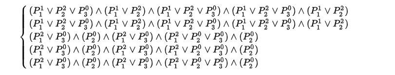
  上述规则就是决策矩阵的每一行的各个cell取交集得到的。然后可以通过集合运算将上面的5条规则化简得到结果如下：
  ${\begin{cases}(P_{1}=1)\to (P_{{4}}=1)\\(P_{2}=2)\to (P_{{4}}=1)\\(P_{1}=2)\land (P_{2}=0)\to (P_{{4}}=1)\\(P_{3}=0)\land (P_{2}=0)\to (P_{{4}}=1)\end{cases}}$
  第一二条规则的support是1，后两条的support是2。（support：在U中满足规则的那些项的个数。）
  这里有些我就省略了，完整的可以看那个维基百科的链接里的内容。
  LEM2
  LEM2是一个比较通用的基于粗糙集的规则提取算法，详细内容可以看我的另外一篇博文。

• Incomplete data
  Rough set theory is useful for rule induction from incomplete data sets. Using this approach we can distinguish between three types of missing attribute values: lost values (the values that were recorded but currently are unavailable), attribute-concept values (these missing attribute values may be replaced by any attribute value limited to the same concept), and “do not care” conditions (the original values were irrelevant). A concept (class) is a set of all objects classified (or diagnosed) the same way.
  Two special data sets with missing attribute values were extensively studied: in the first case, all missing attribute values were lost (Stefanowski and Tsoukias, 2001), in the second case, all missing attribute values were “do not care” conditions (Kryszkiewicz, 1999).
  In attribute-concept values interpretation of a missing attribute value, the missing attribute value may be replaced by any value of the attribute domain restricted to the concept to which the object with a missing attribute value belongs (Grzymala-Busse and Grzymala-Busse, 2007). For example, if for a patient the value of an attribute Temperature is missing, this patient is sick with flu, and all remaining patients sick with flu have values high or very-high for Temperature when using the interpretation of the missing attribute value as the attribute-concept value, we will replace the missing attribute value with high and very-high. Additionally, the characteristic relation, (see, e.g., Grzymala-Busse and Grzymala-Busse, 2007) enables to process data sets with all three kind of missing attribute values at the same time: lost, “do not care” conditions, and attribute-concept values.
  维基中只是generally讲了一下，具体还是得看paper来进行更仔细地了解，暂时还没时间看论文也一下子用不到，之后再说把。

粗糙集的运用
可以用作属性简约（上文中给出的链接中有），以及缺失数据的知识发现等等，论文中有比较具体的描述。

————————————————————————————————
参考文献
就是本文一开始提到的那些参考资料拉。