上节我们简单进行了KNN算法的说明,想想假期结束再回味一下!
Knn算法基本原理:
假设我有如下两个数据集:
dataset = {'black':[ [1,2], [2,3], [3,1] ], 'red':[ [6,5], [7,7], [8,6] ] }
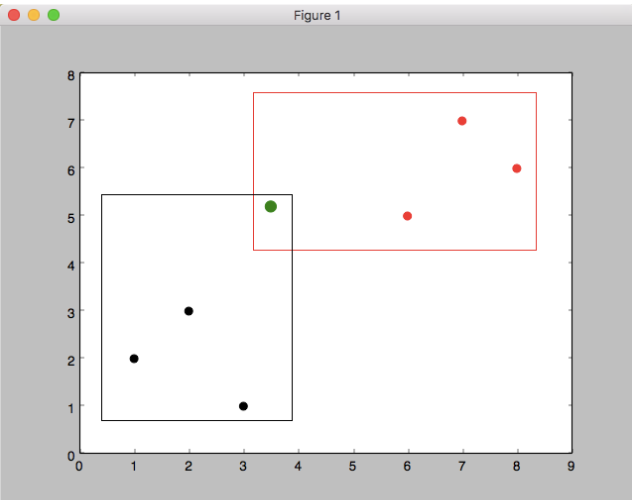
KNN分类算法超级简单:只需使用初中所学的两点距离公式(欧拉距离公式),计算绿点到各组的距离,看绿点和哪组更接近。K代表取离绿点最近的k个点,这k个点如果其中属于红点个数占多数,我们就认为绿点应该划分为红组,反之,则划分为黑组。如果有两组数据(如上图),k值最小应为3(X轴坐标3.5)。
除了K-Nearest Neighbor之外还有其它分组的方法,如Radius-Based Neighbor。此方法后面在做介绍。
实现代码如下:
|
1
2
3
4
5
6
7
8
9
10
11
12
13
14
15
16
17
18
19
20
21
22
23
24
25
26
27
28
29
30
31
32
33
34
35
36
37
38
39
40
41
42
43
44
|
import
math
import
numpy
as
np
from
matplotlib
import
pyplot
from
collections
import
Counter
import
warnings
# k-Nearest Neighbor算法
def
k_nearest_neighbors
(
data
,
predict
,
k
=
5
)
:
if
len
(
data
)
>=
k
:
warnings
.
warn
(
"k is too small"
)
# 计算predict点到各点的距离
distances
=
[
]
for
group
in
data
:
for
features
in
data
[
group
]
:
#euclidean_distance = np.sqrt(np.sum((np.array(features)-np.array(predict))**2)) # 计算欧拉距离,这个方法没有下面一行代码快
euclidean_distance
=
np
.
linalg
.
norm
(
np
.
array
(
features
)
-
np
.
array
(
predict
)
)
distances
.
append
(
[
euclidean_distance
,
group
]
)
sorted_distances
=
[
i
[
1
]
for
i
in
sorted
(
distances
)
]
top_nearest
=
sorted_distances
[
:
k
]
#print(top_nearest) ['red','black','red']
group_res
=
Counter
(
top_nearest
)
.
most_common
(
1
)
[
0
]
[
0
]
confidence
=
Counter
(
top_nearest
)
.
most_common
(
1
)
[
0
]
[
1
]
*
1.0
/
k
# confidences是对本次分类的确定程度,例如(red,red,red),(red,red,black)都分为red组,但是前者显的更自信
return
group_res
,
confidence
if
__name__
==
'__main__'
:
dataset
=
{
'black'
:
[
[
1
,
2
]
,
[
2
,
3
]
,
[
3
,
1
]
]
,
'red'
:
[
[
6
,
5
]
,
[
7
,
7
]
,
[
8
,
6
]
]
}
new_features
=
[
3.5
,
5.2
]
# 判断这个样本属于哪个组
for
i
in
dataset
:
for
ii
in
dataset
[
i
]
:
pyplot
.
scatter
(
ii
[
0
]
,
ii
[
1
]
,
s
=
50
,
color
=
i
)
which_group
,
confidence
=
k_nearest_neighbors
(
dataset
,
new_features
,
k
=
3
)
print
(
which_group
,
confidence
)
pyplot
.
scatter
(
new_features
[
0
]
,
new_features
[
1
]
,
s
=
100
,
color
=
which_group
)
pyplot
.
show
(
)
|
结果如下所示:
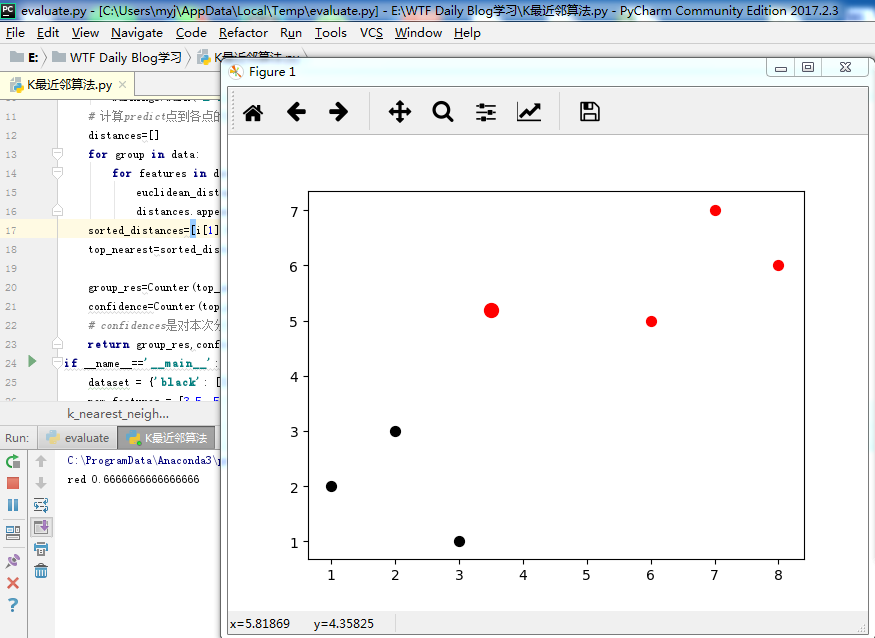
归为红色一类的概率为:0.66666666
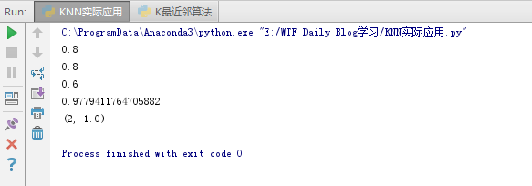
我们使用实际数据进行应用
数据集(Breast Cancer):https://archive.ics.uci.edu/ml/datasets/Breast+Cancer+Wisconsin+%28Original%29
点击download: Data Folder/breast-cancer-wisconsin.data(复制粘贴到txt文件再重命名)
| 代码如下:(if __name__=='__main__':前面代码一样) |
import
math
import
numpy
as
np
from
collections
import
Counter
import
warnings
import
pandas
as
pd
import
random
# k-Nearest Neighbor算法
def
k_nearest_neighbors
(
data
,
predict
,
k
=
5
)
:
if
len
(
data
)
>=
k
:
warnings
.
warn
(
"k is too small"
)
# 计算predict点到各点的距离
distances
=
[
]
for
group
in
data
:
for
features
in
data
[
group
]
:
euclidean_distance
=
np
.
linalg
.
norm
(
np
.
array
(
features
)
-
np
.
array
(
predict
)
)
distances
.
append
(
[
euclidean_distance
,
group
]
)
sorted_distances
=
[
i
[
1
]
for
i
in
sorted
(
distances
)
]
top_nearest
=
sorted_distances
[
:
k
]
group_res
=
Counter
(
top_nearest
)
.
most_common
(
1
)
[
0
]
[
0
]
confidence
=
Counter
(
top_nearest
)
.
most_common
(
1
)
[
0
]
[
1
]
*
1.0
/
k
return
group_res
,
confidence
if __name__=='__main__':
df=pd.read_csv('iris.csv')#加载数据
#print (df.head())
#print(df.shape)
df
.
replace
(
'?'
,
np
.
nan
,
inplace
=
True
)
# -99999
df
.
dropna
(
inplace
=
True
)
# 去掉无效数据
#print(df.shape)
df
.
drop
(
[
'id'
]
,
1
,
inplace
=
True
)#去掉id 这一列(第一列名字为id)
# 把数据分成两部分,训练数据和测试数据
full_data
=
df
.
astype
(
float
)
.
values
.
tolist
(
)
random
.
shuffle
(
full_data
)
test_size
=
0.2
# 测试数据占20%
train_data
=
full_data
[
:
-
int
(
test_size
*
len
(
full_data
)
)
]
test_data
=
full_data
[
-
int
(
test_size
*
len
(
full_data
)
)
:
]
train_set
=
{
2
:
[
]
,
4
:
[
]
}
test_set
=
{
2
:
[
]
,
4
:
[
]
}
for
i
in
train_data
:
train_set
[
i
[
-
1
]
]
.
append
(
i
[
:
-
1
]
)
for
i
in
test_data
:
test_set
[
i
[
-
1
]
]
.
append
(
i
[
:
-
1
]
)
correct
=
0
total
=
0
for
group
in
test_set
:
for
data
in
test_set
[
group
]
:
res
,
confidence
=
k_nearest_neighbors
(
train_set
,
data
,
k
=
5
)
# 你可以调整这个k看看准确率的变化,你也可以使用matplotlib画出k对应的准确率,找到最好的k值
if
group
==
res
:
correct
+=
1
else
:
print
(
confidence
)
total
+=
1
print
(
correct
/
total
)
# 准确率
print
(
k_nearest_neighbors
(
train_set
,
[
4
,
2
,
1
,
1
,
1
,
2
,
3
,
2
,
1
]
,
k
=
5
)
)
# 预测一条记录
结果如下所示:
使用scikit-learn 中K临近算法
代码如下:
import
numpy
as
np
from
sklearn
import
preprocessing
,
cross_validation
,
neighbors
# cross_validation已deprecated,使用model_selection替代
import
pandas
as
pd
df=pd.read_csv('iris.csv')#加载exel数据
#print(df.head())
#print(df.shape)
df
.
replace
(
'?'
,
np
.
nan
,
inplace
=
True
)
# -99999
df
.
dropna
(
inplace
=
True
)
#print(df.shape)
df
.
drop
(
[
'id'
]
,
1
,
inplace
=
True
)
X
=
np
.
array
(
df
.
drop
(
[
'class'
]
,
1
)
)
Y
=
np
.
array
(
df
[
'class'
]
)
X_trian
,
X_test
,
Y_train
,
Y_test
=
cross_validation
.
train_test_split
(
X
,
Y
,
test_size
=
0.2
)
clf
=
neighbors
.
KNeighborsClassifier
(
)
clf
.
fit
(
X_trian
,
Y_train
)
accuracy
=
clf
.
score
(
X_test
,
Y_test
)
print
(
accuracy
)
sample
=
np
.
array
(
[
4
,
2
,
1
,
1
,
1
,
2
,
3
,
2
,
1
]
)
print
(
sample
.
reshape
(
1
,
-
1
)
)
print
(
clf
.
predict
(
sample
.
reshape
(
1
,
-
1
)
)
)
结果如下:(里面有个警告但不妨碍结果)
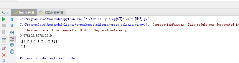
scikit-learn中的算法和我们上面实现的算法原理完全一样,只是它的效率更高,支持的参数更全。 (以上内容学习于大熊猫) |