直方图的比较:
应用:
通过直方图粗略比较图像的相似性(通过相关性、卡方等数学参量),往往用于第一阶段的图像识别。
代码:
直方图的横坐标为颜色空间,纵坐标为该颜色的像素点的个数。由于一个RGB像素点由3个颜色空间决定,即它的种类有256* 256* 256种;我们将其色彩空间进行划分,将R,G,B的Binsize设置为16,这时候每个颜色通道有16个bins,因此横坐标range为0—16* 16* 16.(这样子理解:将RGB都是为一个维度,它们决定的正整数点的个数为256 * 256 * 256 ,然后我们将它们降低维度!)
- 生成一张直方图:
#in order to get a RGB-image Histogram
def create_rgb_hist(image):
    h, w, c = image.shape;
    rgbHist = np.zeros([16*16*16, 1], np.float32);
    #use 1 to initialize the height of rbghist[], but you must use rgbHist[, 0] to access a number.
    bsize = 256/16;
    for row in range(h):
        for col in range(w):
            b = image[row, col, 0];
            g = image[row, col, 1];
            r = image[row, col, 2];
            index = np.int(b/bsize)*16*16 + np.int(g/bsize)*16 + np.int(r/bsize);
            regHist[np.int(index), 0] = regHist[np.int(index), 0] + 1;
            #use 0 to represent the index
    return rebHist;
- 直方图比较(3中比较参数):
def hist_compare(image1, image2):
    hist1 = create_rgb_hist(image1);
    hist2 = create_rgb_hist(image2);
    match1 = cv.compareHist(hist1, hist2, cv.HISTCMP_BHATTACHARYYA);#巴氏距离
    match2 = cv.compareHist(hist1, hist2, cv.HISTCMP_CORREL);#相关性
    match3 = cv.compareHist(hist1, hist2, cv.HISTCMP_CHISQR);#卡方
    print("巴氏距离: %s ,相关性: %s ,卡方: %s"%(match1, match2, match3));
直方图的反向投影:
2D直方图的构建:
def hist2d_demo(image):
    hsv = cv.cvtColor(image, cv.COLOR_BGR2HSV);
    hist = cv.calcHist([image], [0, 1], None, [180, 256], [0, 180, 0, 256]);
    plt.imshow(hist, interpolation = 'nearest');
    plt.title("2D Histogram");
    plt.show();
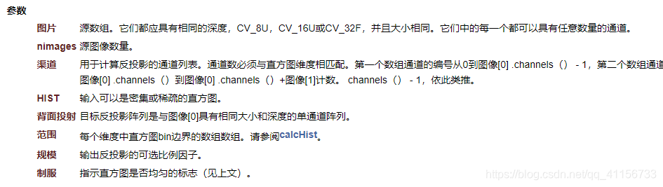
通过反向直方图完成目标提取:
-
做直方图反向投影,必须把图像颜色空间转化为HSV空间:因为BGR直方图我们只能三个通道分别计算,计算后也没法合在一起,也就是不能把图片作为一个整体来比较,而H-S就可以将图片作一个整体对比,所以这里用H-S直方图来作反向投影!(咋也不知道对不对~)
-
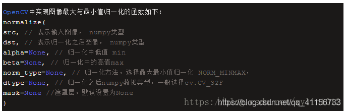
图像的标准化及归一化
只是用于将图像归一化而已,无论是针对二维直方图,或者是一般图像。
原图与归一化之后的运行结果完全一致,说明归一化不会改变图像本身的信息存储,但是通过打印出来的像素值可以发现,取值范围从0~255已经转化为0~1之间了,这个对于后续的神经网络或者卷积神经网络处理有很大的好处,tensorflow官方给出mnist数据集,全部采用了归一化之后的结果作为输入图像数据来演示神经网络与卷积神经网络。
-
代码:
def back_projection_demo():
    sample = cv.imread("E:/picture/sample.png");
    target = cv.imread("E:/picture/target.jpg");#待检测目标
    sample_hsv = cv.cvtColor(sample, cv.COLOR_BGR2HSV);
    target_hsv = cv.cvtColor(target, cv.COLOR_BGR2HSV);

    #show image
    cv.imshow("sample", sample);
    cv.imshow("target", target);

    #show the image before normalization
    sampleHist = cv.calcHist([sample_hsv], [0, 1], None, [180, 256], [0, 180, 0, 256]);
    #可以通过调节histsize([180, 256]且要设置为256的因子)来使得图片避免碎片化
    plt.imshow(sampleHist, interpolation = 'nearest');
    plt.title("2D Histogram before normalize");
    plt.show();
    print(sampleHist);

    #show the image after normalization
    cv.normalize(sampleHist, sampleHist, 0, 255, cv.NORM_MINMAX);
    plt.imshow(sampleHist, interpolation = 'nearest');
    plt.title("2D Histogram after normalize");
    plt.show();
    print("------------------------------------");
    print(sampleHist);

    dst = cv.calcBackProject([target_hsv], [0, 1], sampleHist, [0, 180, 0, 256], 1);
    cv.imshow("backProjection_demo", dst);
可以通过调节Histszie(也即bins的个数),来设置图片还原的清晰度。因为,直方图的bins越多,直方图分的越西,会产生图片的碎片化。因此我们不要将Histsize设置地太小!!!
