一、K-Means算法和Mini Batch K-Means算法比较

# Author:yifan

import time

import numpy as np

import matplotlib.pyplot as plt

import matplotlib as mpl

from sklearn.cluster import MiniBatchKMeans,KMeans

from sklearn.metrics.pairwise import pairwise_distances_argmin

from sklearn.datasets.samples_generator import make_blobs

## 设置属性防止中文乱码

mpl.rcParams['font.sans-serif'] = [u'SimHei']

mpl.rcParams['axes.unicode_minus']=False

#初始化三个中心

centers = [[1,1],[-1,-1],[1,-1]]

clusters = len(centers) #聚类的数目为3

#产生3000组二维的数据，中心是意思三个中心点，标准差是.7

X,Y = make_blobs(n_samples=28000,centers=centers,cluster_std=0.7,random_state=28)

#构建kmeans算法

k_means = KMeans(init='k-means++',n_clusters=clusters,random_state=28)

t0 = time.time() #current time

k_means.fit(X) #trainning mode

km_batch = time.time() - t0 #the spend of trainning mode

print("K-means算法所需要的时间：%.4fs" % km_batch)

#构建MiniBatchKMeans算法

batch_size = 100

mbk = MiniBatchKMeans(init='k-means++',n_clusters=clusters,batch_size=batch_size,random_state=28)

t0=time.time()

mbk.fit(X)

mbk_batch = time.time()-t0 ##the spend of trainning mode

print ("Mini Batch K-Means算法模型训练消耗时间:%.4fs" % mbk_batch)

#预测结果

km_y_hat = k_means.predict(X)

mbkm_y_hat = mbk.predict(X)

print(km_y_hat[:10])

print(mbkm_y_hat[:10])

print(k_means.cluster_centers_)

print(mbk.cluster_centers_)

##获取聚类中心点并聚类中心点进行排序

k_means_cluster_centers = k_means.cluster_centers_ #输出kmeans聚类中心点

mbk_means_cluster_centers = mbk.cluster_centers_ #输出mbk聚类中心点

print ("K-Means算法聚类中心点:\ncenter=", k_means_cluster_centers)

print ("Mini Batch K-Means算法聚类中心点:\ncenter=", mbk_means_cluster_centers)

order = pairwise_distances_argmin(k_means_cluster_centers, mbk_means_cluster_centers) #array([1, 2, 0], dtype=int64)

#方便后面画图

#画图

plt.figure(figsize=(12,6),facecolor='w')

plt.subplots_adjust(left=0.05,right=0.95,bottom=0.05,top=0.9)

cm = mpl.colors.ListedColormap(['#FFC2CC', '#C2FFCC', '#CCC2FF'])

cm2 = mpl.colors.ListedColormap(['#FF0000', '#00FF00', '#0000FF'])

#子图1：原始数据

plt.subplot(221)

plt.scatter(X[:,0],X[:,1],c=Y,s=6,cmap = cm,edgecolors='none')

plt.title(u'原始数据分布图')

plt.xticks(())

plt.yticks(())

plt.grid(True)

#子图2：K-Means算法聚类结果图

plt.subplot(222)

plt.scatter(X[:,0],X[:,1],c=km_y_hat,s=6,cmap=cm,edgecolors='none')

plt.scatter(k_means_cluster_centers[:,0], k_means_cluster_centers[:,1],c=range(clusters),s=60,cmap=cm2,edgecolors='none')

plt.title(u'K-Means算法聚类图')

plt.xticks(())

plt.yticks(())

plt.text(-3.8, 3, 'train time: %.2fms' % (km_batch*1000))

plt.grid(True)

#子图3:Mini Batch K-Means算法聚类结果图

plt.subplot(223)

plt.scatter(X[:,0], X[:,1], c=km_y_hat, s=6, cmap=cm,edgecolors='none')

plt.scatter(mbk_means_cluster_centers[:,0],mbk_means_cluster_centers[:,1],c=range(clusters),s=60,cmap=cm2,edgecolors='none')

plt.title(u'Mini Batch K-Means算法聚类结果图')

plt.xticks(())

plt.yticks(())

plt.text(-3.8, 3, 'train time: %.2fms' % (mbk_batch*1000))

plt.grid(True)

#统计不同的数据个数

different = list(map(lambda x:(x!=0) & (x!=1) &(x!=2),mbkm_y_hat))

for k in range(clusters):

different += ((km_y_hat == k) != (mbkm_y_hat == order[k]))

idendic = np.logical_not(different)

different_nodes = len(list(filter(lambda x:x, different)))

#根据上面的统计，画出预测异同点

plt.subplot(224)

#相同部分；

plt.plot(X[idendic,0],X[idendic,1],'w',markerfacecolor = '#bbbbbb',marker='.')

#不相同部分；

plt.plot(X[different, 0], X[different, 1], 'w', markerfacecolor='m', marker='.')

plt.title(u'Mini Batch K-Means和K-Means算法预测结果不同的点')

plt.xticks(())

plt.yticks(())

plt.text(-3.8, 2, 'different nodes: %d' % (different_nodes))

plt.show()

结果：

K-means算法所需要的时间：0.1945s

Mini Batch K-Means算法模型训练消耗时间:0.0728s

[2 1 2 0 0 1 2 2 0 0]

[1 0 1 2 2 0 1 1 2 2]

[[ 1.05236122 -1.06341323]

[ 1.00290173 1.03159141]

[-1.03255552 -1.00256646]]

[[ 0.93636615 1.04956555]

[-0.96042372 -1.04840814]

[ 1.18516308 -1.00675752]]

K-Means算法聚类中心点:

center= [[ 1.05236122 -1.06341323]

[ 1.00290173 1.03159141]

[-1.03255552 -1.00256646]]

Mini Batch K-Means算法聚类中心点:

center= [[ 0.93636615 1.04956555]

[-0.96042372 -1.04840814]

[ 1.18516308 -1.00675752]]

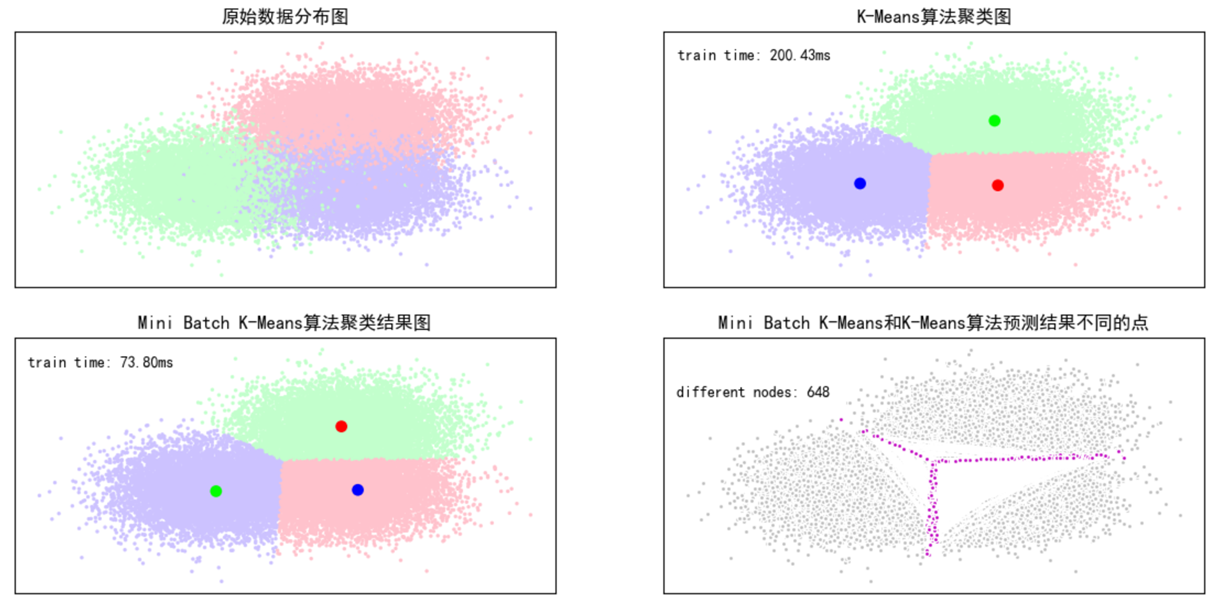
Mini Batch K-Mean效果差一点，但是速度快。

二、层次聚类(BIRCH)算法参数比较

# Author:yifan

from itertools import cycle

from time import time

import numpy as np

import matplotlib as mpl

import matplotlib.pyplot as plt

import matplotlib.colors as colors

from sklearn.preprocessing import StandardScaler

from sklearn.cluster import Birch

from sklearn.datasets.samples_generator import make_blobs

## 设置属性防止中文乱码

mpl.rcParams['font.sans-serif'] = [u'SimHei']

mpl.rcParams['axes.unicode_minus'] = False

## 产生模拟数据

xx = np.linspace(-22, 22, 10)

yy = np.linspace(-22, 22, 10)

xx, yy = np.meshgrid(xx, yy)

n_centres = np.hstack((np.ravel(xx)[:, np.newaxis],np.ravel(yy)[:, np.newaxis]))

#产生10万条特征属性是2，类别是100,符合高斯分布的数据集

X, y = make_blobs(n_samples=100000,n_features=2, centers=n_centres, random_state=28)

#创建不同的参数（簇直径）Birch层次聚类

birch_models = [

Birch(threshold=1.7, n_clusters=None), #运行的函数

Birch(threshold=0.5, n_clusters=None),

Birch(threshold=1.7, n_clusters=100)]

#threshold：簇直径的阈值， branching_factor：大叶子个数

#我们也可以加参数来试一下效果，比如加入分支因子branching_factor，给定不同的参数值，看聚类的结果

## 画图

final_step = [u'直径=1.7;n_lusters=None', u'直径=0.5;n_clusters=None', u'直径=1.7;n_lusters=100']

plt.figure(figsize=(12, 8), facecolor='w')

plt.subplots_adjust(left=0.02, right=0.98, bottom=0.1, top=0.9)

colors_ = cycle(colors.cnames.keys())

cm = mpl.colors.ListedColormap(colors.cnames.keys())

for ind, (birch_model, info) in enumerate(zip(birch_models, final_step)):

t = time()

birch_model.fit(X)

time_ = time() - t

# 获取模型结果（label和中心点）

labels = birch_model.labels_

centroids = birch_model.subcluster_centers_

n_clusters = len(np.unique(centroids))

print("Birch算法，参数信息为：%s；模型构建耗时为:%.3f秒；聚类中心数目:%d" % (info, time_, len(np.unique(labels))))

## 画图

subinx = 222 + ind

plt.subplot(subinx)

for this_centroid, k, col in zip(centroids, range(n_clusters), colors_):

mask = labels == k

plt.plot(X[mask, 0], X[mask, 1], 'w', markerfacecolor=col, marker='.')

if birch_model.n_clusters is None:

plt.plot(this_centroid[0], this_centroid[1], '*', markerfacecolor=col, markeredgecolor='k', markersize=2)

plt.ylim([-25, 25])

plt.xlim([-25, 25])

plt.title(u'Birch算法%s，耗时%.3fs' % (info, time_))

plt.grid(False)

## 原始数据集显示

plt.subplot(221)

plt.scatter(X[:, 0], X[:, 1], c=y, s=1, cmap=cm, edgecolors='none')

plt.ylim([-25, 25])

plt.xlim([-25, 25])

plt.title(u'原始数据')

plt.grid(False)

plt.show()

结果：

Birch算法，参数信息为：直径=1.7;n_lusters=None；模型构建消耗时间为:3.250秒；聚类中心数目:171

Birch算法，参数信息为：直径=0.5;n_clusters=None；模型构建消耗时间为:8.347秒；聚类中心数目:3205

Birch算法，参数信息为：直径=1.7;n_lusters=100；模型构建消耗时间为:3.333秒；聚类中心数目:100

三、DBSCAN算法

# Author:yifan

import numpy as np

import matplotlib as mpl

import matplotlib.pyplot as plt

import sklearn.datasets as ds

import matplotlib.colors

from sklearn.cluster import DBSCAN

from sklearn.preprocessing import StandardScaler

## 设置属性防止中文乱码及拦截异常信息

mpl.rcParams['font.sans-serif'] = [u'SimHei']

mpl.rcParams['axes.unicode_minus'] = False

### 创建模拟数据

N = 1000

centers = [[1, 2], [-1, -1], [1, -1], [-1, 1]]

data1, y1 = ds.make_blobs(N, n_features=2, centers=centers, cluster_std=(1,0.75, 0.5,0.25), random_state=0)

data1 = StandardScaler().fit_transform(data1)

params1 = ((0.15, 5), (0.2, 10), (0.2, 15), (0.3, 5), (0.3, 10), (0.3, 15)) #六种参数，后面画出六个图例

t = np.arange(0, 2 * np.pi, 0.1)

data2_1 = np.vstack((np.cos(t), np.sin(t))).T

data2_2 = np.vstack((2*np.cos(t), 2*np.sin(t))).T

data2_3 = np.vstack((3*np.cos(t), 3*np.sin(t))).T

data2 = np.vstack((data2_1, data2_2, data2_3))

y2 = np.vstack(([0] * len(data2_1), [1] * len(data2_2), [2] * len(data2_3))).reshape(-1,)

params2 = ((0.5, 3), (0.5, 5), (0.5, 10), (1., 3), (1., 10), (1., 20))

datasets = [(data1, y1,params1), (data2, y2,params2)]

def expandBorder(a, b):

d = (b - a) * 0.1

return a-d, b+d

colors = ['r', 'g', 'b', 'y', 'c', 'k']

cm = mpl.colors.ListedColormap(colors)

for i, (X, y, params) in enumerate(datasets):

x1_min, x2_min = np.min(X, axis=0)

x1_max, x2_max = np.max(X, axis=0)

x1_min, x1_max = expandBorder(x1_min, x1_max)

x2_min, x2_max = expandBorder(x2_min, x2_max)

plt.figure(figsize=(12, 8), facecolor='w')

plt.suptitle(u'DBSCAN聚类-数据%d' % (i + 1), fontsize=18)

plt.subplots_adjust(top=0.9, hspace=0.35)

for j, param in enumerate(params):

eps, min_samples = param

model = DBSCAN(eps=eps, min_samples=min_samples)

# eps 半径，控制邻域的大小，值越大，越能容忍噪声点，值越小，相比形成的簇就越多

# min_samples 原理中所说的M，控制哪个是核心点，值越小，越可以容忍噪声点，越大，就更容易把有效点划分成噪声点

model.fit(X)

y_hat = model.labels_

unique_y_hat = np.unique(y_hat)

n_clusters = len(unique_y_hat) - (1 if -1 in y_hat else 0)

print("类别:", unique_y_hat, "；聚类簇数目:", n_clusters)

core_samples_mask = np.zeros_like(y_hat, dtype=bool)

core_samples_mask[model.core_sample_indices_] = True

## 开始画图

plt.subplot(3, 3, j + 1)

for k, col in zip(unique_y_hat, colors):

if k == -1:

col = 'k'

class_member_mask = (y_hat == k)

xy = X[class_member_mask & core_samples_mask]

plt.plot(xy[:, 0], xy[:, 1], 'o', markerfacecolor=col, markeredgecolor='k', markersize=14)

xy = X[class_member_mask & ~core_samples_mask]

plt.plot(xy[:, 0], xy[:, 1], 'o', markerfacecolor=col, markeredgecolor='k', markersize=6)

plt.xlim((x1_min, x1_max))

plt.ylim((x2_min, x2_max))

plt.grid(True)

plt.title('$\epsilon$ = %.1f m = %d，聚类簇数目：%d' % (eps, min_samples, n_clusters), fontsize=12)

## 原始数据显示

plt.subplot(3, 3, 7)

plt.scatter(X[:, 0], X[:, 1], c=y, s=30, cmap=cm, edgecolors='none')

plt.xlim((x1_min, x1_max))

plt.ylim((x2_min, x2_max))

plt.title('原始数据，聚类簇数目:%d' % len(np.unique(y)))

plt.grid(True)

plt.show()

类别: [-1 0 1 2 3 4 5 6 7 8 9 10 11 12 13 14 15] ；聚类簇数目: 16

类别: [-1 0 1 2 3 4] ；聚类簇数目: 5

类别: [-1 0 1 2] ；聚类簇数目: 3

类别: [-1 0] ；聚类簇数目: 1

类别: [0 1 2] ；聚类簇数目: 3

类别: [-1 0 1] ；聚类簇数目: 2

类别: [-1 0] ；聚类簇数目: 1

类别: [0] ；聚类簇数目: 1

类别: [-1 0] ；聚类簇数目: 1

【ML-7】聚类算法-实例代码

目录

一、K-Means算法和Mini Batch K-Means算法比较

结果：

二、层次聚类(BIRCH)算法参数比较

结果：

三、DBSCAN算法

猜你喜欢