从一个简单的数据集学习Logistic Regression

Logistic Regression

Logistic Regression是一种被广泛使用的分类算法，通过训练数据中的正负样本，学习样本特征到样本标签之间的假设函数。

通常用于将数据映射到不同类别的函数成为阈值函数，常用的阈值函数为Sigmoid函数，形式为：
$f(x)=\frac{1}{1+e^{-x}}$
Sigmoid函数的图像：

在这里插入图片描述
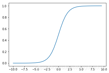
从Sigmoid的图像可以看出函数的值域为(0,1),在0附近变化比较明显

Sigmoid函数的python代码：

def sig(x):
    '''Sigmoid函数
    input:  x(mat):feature * w
    output: sigmoid(x)(mat):Sigmoid值
    '''
    return 1.0 / (1 + np.exp(-x))

因此对于输入向量X，其属于正例和反例的概率为：
$正例的概率： P(y=1|X,W,b)=\frac{1}{1+e^{-（WX+b）}}\\反例的概率： P(y=1|X,W,b)=\frac{e^{-(WX+b)}}{1+e^{-（WX+b）}}$
对于Logistic Regression算法来说，如何定义W和b使得算法最优？(什么是最优)

为了求解最优的权重矩阵W和偏置向量b，需要定义损失函数

对于上述的Logistic Regression算法，属于类别 y 的概率是
$P(y|X,W,b)=\sigma(WX+b)^y(1-\sigma(WX+b))^{1-y}$
其中 σ 表示的是Sigmoid函数。

在此用极大似然法进行估计。假设训练数据集有m个训练样本{{X1,Y1},{X2,Y2},……{Xn,Yn}},则其似然函数为：
$L_{W,b}=\prod_{i=1}^{m}[h_{W,b}(X^{i})^{y^i}(1-h_{W,b}(X^i))^{1-y^i}]$
其中的假设函数
$h_{W,b}(X^i)=\sigma(WX^i+b)$
对于似然函数的极大值的求解，通常使用Log似然函数，在Logistic Regression算法中，通常是将负的Log似然函数作为其损失函数，则只需要计算其极小值就行
$l_{W,b}=-\frac{1}{m}logL_{W,b}$
可以通过梯度下降法求得损失函数的最小值以及其对应的参数值。

利用梯度下降法训练Logistic Regression模型：

上述问题的梯度：
$\bigtriangledown _{W_j}(l_{w,b})=-\frac{1}{m}\sum_{i=1}^{m}({y^i-h_{W,b}(X^i)})x_j^i\\\bigtriangledown _{b}(l_{w,b})=-\frac{1}{m}\sum_{i=1}^{m}({y^i-h_{W,b}(X^i)})\\其中x_j^i表示样本X^i的第j个分量$
取w0=b，且将偏置项的变量x0设置位1，则上述可合并为：
$\bigtriangledown _{W_j}(l_{w,b})=-\frac{1}{m}\sum_{i=1}^{m}({y^i-h_{W,b}(X^i)})x_j^i$
根据梯度下降法，得到的更新公式：
$W_j=W_j-\alpha\bigtriangledown_{W_j}(l_w,b)$
可以用代码表示出具体的梯度下降法过程：

def lr_train_bgd(feature, label, maxCycle, alpha):
    '''利用梯度下降法训练LR模型
    input:  feature(mat)特征
            label(mat)标签
            maxCycle(int)最大迭代次数
            alpha(float)学习率
    output: w(mat):权重
    '''
    n = np.shape(feature)[1]  # 特征个数
    w = np.mat(np.ones((n, 1)))  # 初始化权重
    i = 0
    while i <= maxCycle:  # 在最大迭代次数的范围内
        i += 1  # 当前的迭代次数
        h = sig(feature * w)  # 计算Sigmoid值
        err = label - h
        if i % 100 == 0:
            print ("\t---------iter=" + str(i) + \
            " , train error rate= " + str(error_rate(h, label)))
        w = w + alpha * feature.T * err  # 权重修正
    return w

计算损失值的函数的python代码：

扫描二维码关注公众号，回复： 9114855 查看本文章

def error_rate(h, label):
    '''计算当前的损失函数值
    input:  h(mat):预测值
            label(mat):实际值
    output: err/m(float):错误率
    '''
    m = np.shape(h)[0]
    
    sum_err = 0.0
    for i in range(m):
        if h[i, 0] > 0 and (1 - h[i, 0]) > 0:
            sum_err -= (label[i,0] * np.log(h[i,0]) + \
                        (1-label[i,0]) * np.log(1-h[i,0]))
        else:
            sum_err -= 0
    return sum_err / m

基于上述操作，可以完成Logistic Regression算法的实践：

利用训练样本训练模型
利用训练好的模型对新样本进行预测

训练模型的主函数:

if __name__ == "__main__":
    # 1、导入训练数据
    print ("---------- 1.load data ------------")
    feature, label = load_data("data.txt")
    # 2、训练LR模型
    print ("---------- 2.training ------------")
    w = lr_train_bgd(feature, label, 1000, 0.01)
    # 3、保存最终的模型
    print ("---------- 3.save model ------------")
    save_model("weights", w)

主要步骤为：

导入训练数据
利用梯度下降法对训练数据进行训练
将权重输出到文件weight中

导入数据的代码：

def load_data(file_name):
    '''导入训练数据
    input:  file_name(string)训练数据的位置
    output: feature_data(mat)特征
            label_data(mat)标签
    '''
    f = open(file_name)  # 打开文件
    feature_data = []
    label_data = []
    for line in f.readlines():
        feature_tmp = []
        lable_tmp = []
        lines = line.strip().split("\t")
        feature_tmp.append(1)  # 偏置项
        for i in range(len(lines) - 1):
            feature_tmp.append(float(lines[i]))
        lable_tmp.append(float(lines[-1]))
        
        feature_data.append(feature_tmp)
        label_data.append(lable_tmp)
    f.close()  # 关闭文件
    return np.mat(feature_data), np.mat(label_data)

保存最终模型的代码：

def save_model(file_name, w):
    '''保存最终的模型
    input:  file_name(string):模型保存的文件名
            w(mat):LR模型的权重
    '''
    m = np.shape(w)[0]
    f_w = open(file_name, "w")
    w_array = []
    for i in range(m):
        w_array.append(str(w[i, 0]))
    f_w.write("\t".join(w_array))
    f_w.close()

运行可知具体的训练过程：

---------- 1.load data ------------
---------- 2.training ------------
        ---------iter=100 , train error rate= 0.0011343552118725237
        ---------iter=200 , train error rate= 0.0009477843077847493
        ---------iter=300 , train error rate= 0.0008150655965653218
        ---------iter=400 , train error rate= 0.0007156807636573261
        ---------iter=500 , train error rate= 0.000638391025133774
        ---------iter=600 , train error rate= 0.0005765152961049218
        ---------iter=700 , train error rate= 0.000525828329858299
        ---------iter=800 , train error rate= 0.0004835251428600975
        ---------iter=900 , train error rate= 0.0004476693385107426
        ---------iter=1000 , train error rate= 0.00041688036889435637
---------- 3.save model ------------

可以看到对于训练集的错误率一直在降低。

通过训练后得到的Logistic Regression的模型的权重为

1.3941777508748279	4.527177129107412	-4.793981623770905

对新数据进行预测：

包括导入模型
导入测试集
对数据集进行预测
保留结果

测试的代码如下：

# coding:UTF-8
import numpy as np
from lr_train import sig

def load_weight(w):
    '''导入LR模型
    input:  w(string)权重所在的文件位置
    output: np.mat(w)(mat)权重的矩阵
    '''
    f = open(w)
    w = []
    for line in f.readlines():
        lines = line.strip().split("\t")
        w_tmp = []
        for x in lines:
            w_tmp.append(float(x))
        w.append(w_tmp)    
    f.close()
    return np.mat(w)

def load_data(file_name, n):
    '''导入测试数据
    input:  file_name(string)测试集的位置
            n(int)特征的个数
    output: np.mat(feature_data)(mat)测试集的特征
    '''
    f = open(file_name)
    feature_data = []
    for line in f.readlines():
        feature_tmp = []
        lines = line.strip().split("\t")
        # print lines[2]
        if len(lines) != n - 1:
            continue
        feature_tmp.append(1)
        for x in lines:
            # print x
            feature_tmp.append(float(x))
        feature_data.append(feature_tmp)
    f.close()
    return np.mat(feature_data)

def predict(data, w):
    '''对测试数据进行预测
    input:  data(mat)测试数据的特征
            w(mat)模型的参数
    output: h(mat)最终的预测结果
    '''
    h = sig(data * w.T)#sig
    m = np.shape(h)[0]
    for i in range(m):
        if h[i, 0] < 0.5:
            h[i, 0] = 0.0
        else:
            h[i, 0] = 1.0
    return h

def save_result(file_name, result):
    '''保存最终的预测结果
    input:  file_name(string):预测结果保存的文件名
            result(mat):预测的结果
    '''
    m = np.shape(result)[0]
    #输出预测结果到文件
    tmp = []
    for i in range(m):
        tmp.append(str(result[i, 0]))
    f_result = open(file_name, "w")
    f_result.write("\t".join(tmp))
    f_result.close()    

if __name__ == "__main__":
    # 1、导入LR模型
    print ("---------- 1.load model ------------")
    w = load_weight("weights")
    n = np.shape(w)[1]
    # 2、导入测试数据
    print ("---------- 2.load data ------------")
    testData = load_data("test_data", n)
    # 3、对测试数据进行预测
    print ("---------- 3.get prediction ------------")
    h = predict(testData, w)#进行预测
    # 4、保存最终的预测结果
    print ("---------- 4.save prediction ------------")
    save_result("result", h)

数据集和测试数据集：
https://pan.baidu.com/s/1i-0qomeuKqA4I2fcfEuutg

coding丁

发布了68 篇原创文章 · 获赞 36 · 访问量 1万+

私信关注

从一个简单的数据集学习Logistic Regression

Logistic Regression

猜你喜欢