假设共有m个样本：当 Mini-batch = 1 时，为随机梯度下降; 当 Mini-batch = m 时，为 batch 梯度下降; 当 1 < Mini-batch < m 时，为 Mini-batch 梯度下降。通常情况下 mini-batch 取 $2^n$ （如：64， 128 等）。
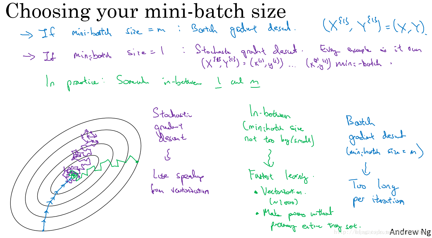在这里插入图片描述该图来自吴恩达深度学习视频教程。从中可以看出 Mini-batch 收敛速度快、波动小等优点。数据集来源：链接: https://pan.baidu.com/s/1_GY48DuWrzBnDfuGTv7Bbg 提取码: 2ksj

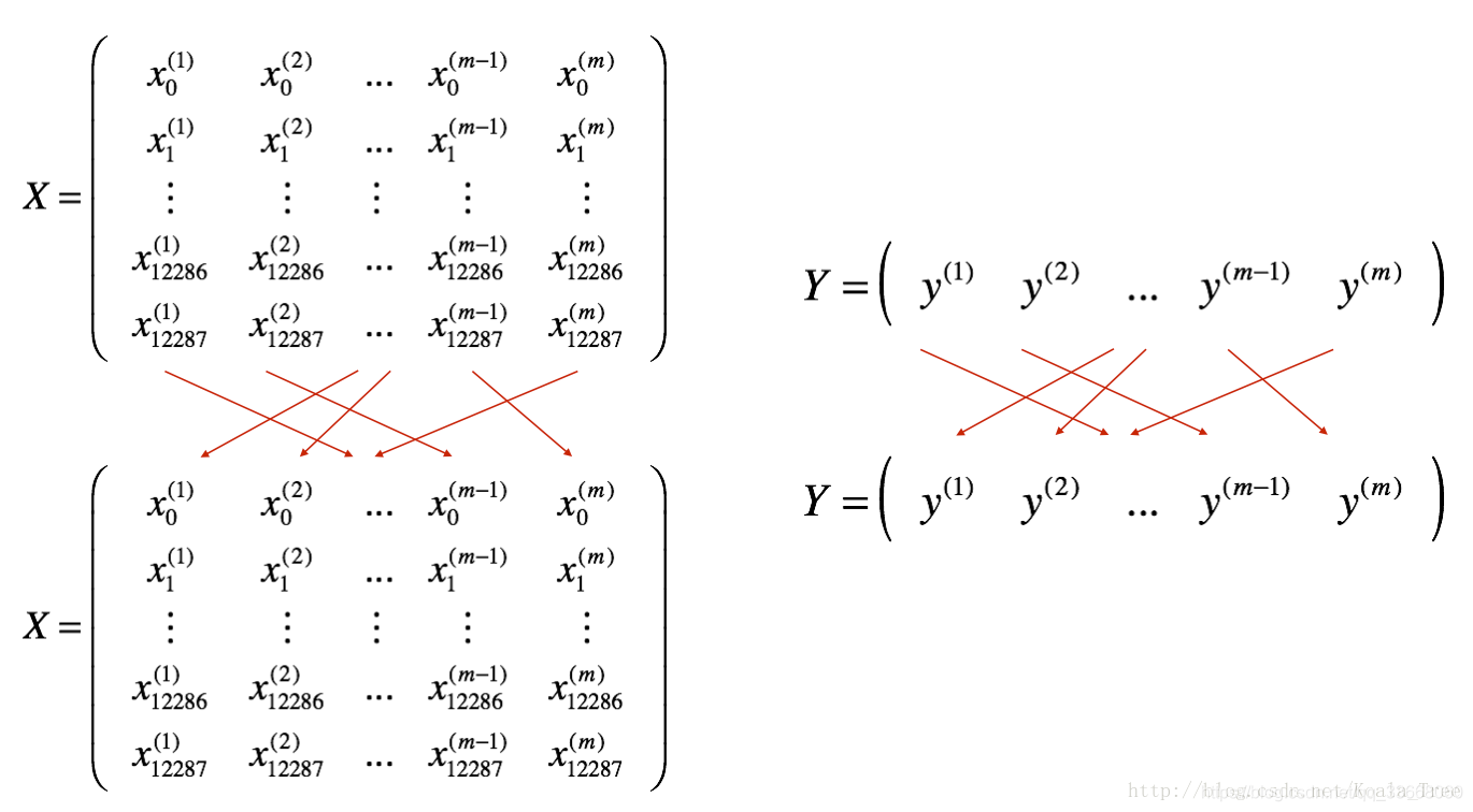
在进行 mini_batch 之前使用 np.random.permutation() 函数数据集打乱，如下图所示。下图中上层是原始数据集的顺序，下层是shuffle操作后的乱序。采用的函数是：
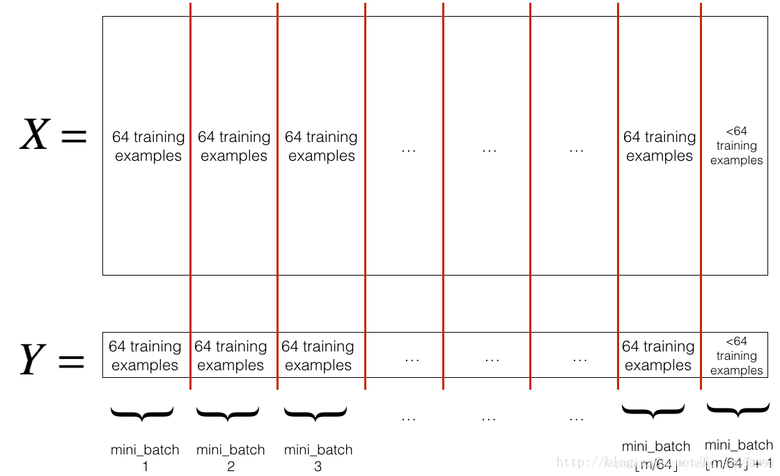
在这里插入图片描述然后利用 shuffle 操作，按照 mini_batch_size 分割整个数据集，代码形式：

first_mini_batch_X = shuffled_X[:, 0 : mini_batch_size]
second_mini_batch_X = shuffled_X[:, mini_batch_size : 2 * mini_batch_size]
...
...

在这里插入图片描述
数据集mini_batch的具体算法实现（python）：

import numpy as np
import h5py
import math


# 定义数据集，，，读者下载好数据集后  需要将 此处的 train_dataset 和 test_dataset 改为自己的数据地址文件夹
def load_dataset():
    train_dataset = h5py.File('/home/zwb/Logistic_Regression/train_catvnoncat.h5', "r")
    train_set_x_orig = np.array(train_dataset["train_set_x"][:]) # your train set features
    train_set_y_orig = np.array(train_dataset["train_set_y"][:]) # your train set labels

    test_dataset = h5py.File('/home/zwb/Logistic_Regression/test_catvnoncat.h5', "r")
    test_set_x_orig = np.array(test_dataset["test_set_x"][:]) # your test set features
    test_set_y_orig = np.array(test_dataset["test_set_y"][:]) # your test set labels

    classes = np.array(test_dataset["list_classes"][:]) # the list of classes
    
    train_set_y_orig = train_set_y_orig.reshape((1, train_set_y_orig.shape[0]))
    test_set_y_orig = test_set_y_orig.reshape((1, test_set_y_orig.shape[0]))
    
    return train_set_x_orig, train_set_y_orig, test_set_x_orig, test_set_y_orig, classes

# 定义mini_batch函数
def random_mini_batches(X, Y, mini_batch_size=64, seed=0):
    np.random.seed(seed)
    m = X.shape[1]
    mini_batches = []
    
    # 利用 np.random.permutation()函数将整个数据集打乱
    permutation = list(np.random.permutation(m))
    shuffled_X = X[:, permutation]
    shuffled_Y = Y[:, permutation].reshape((1, m))
    num_complete_minibatches = math.floor(m/mini_batch_size) #计算有多少个mini_batch
    
    # 构建每个 mini_batch, 并将每一组的mini_batch 存放到 mini_batches 中
    for k in range(0, num_complete_minibatches):  #完整的 mini_batch
        mini_batch_X = shuffled_X[:, k*mini_batch_size:(1+k)*mini_batch_size]
        mini_batch_Y = shuffled_Y[:, k*mini_batch_size:(1+k)*mini_batch_size]
        mini_batch = (mini_batch_X, mini_batch_Y)
        mini_batches.append(mini_batch)
        
    if m % mini_batch_size != 0:  #剩余不足64的数据
        mini_batch_X = shuffled_X[:, num_complete_minibatches*mini_batch_size:m]
        mini_batch_Y = shuffled_Y[:, num_complete_minibatches*mini_batch_size:m]
        mini_batch = (mini_batch_X, mini_batch_Y)
        mini_batches.append(mini_batch)
        
    return mini_batches

train_x, train_y, test_x, test_y, classes = load_dataset()
train_x = train_x.reshape(train_x.shape[0], -1).T  #将每个数据学成列的形式
mini_batches = random_mini_batches(train_x, train_y, mini_batch_size=64, seed=0)

for i in range(len(mini_batches)):
    print ("Shape of the {} mini_batch_X: {}" .format(i, mini_batches[i][0].shape))
    print ("Shape of the {} mini_batch_Y: {}" .format(i, mini_batches[i][1].shape))

结果：
Shape of the 0 mini_batch_X: (12288, 64)
Shape of the 0 mini_batch_Y: (1, 64)
Shape of the 1 mini_batch_X: (12288, 64)
Shape of the 1 mini_batch_Y: (1, 64)
Shape of the 2 mini_batch_X: (12288, 64)
Shape of the 2 mini_batch_Y: (1, 64)
Shape of the 3 mini_batch_X: (12288, 17)
Shape of the 3 mini_batch_Y: (1, 17)

（2）数据集的归一化处理

数据集的归一化处理就是将输入数据进行归一化操作，这样做的目的是将数据集中样本的分布在同一个概率分布空间中。
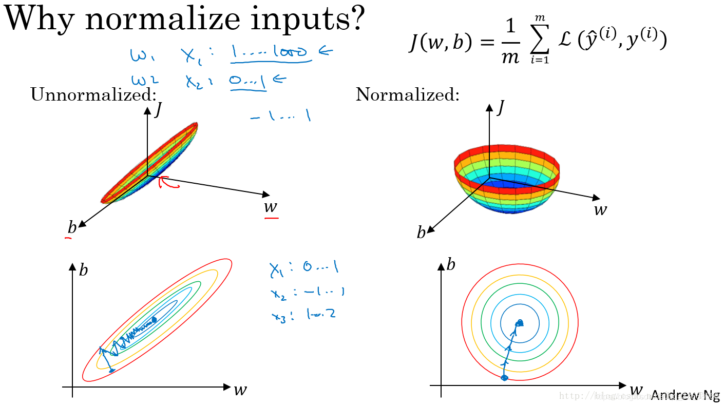在这里插入图片描述从图上可以看出，经过归一化处理后的损失函数，无论起始点在哪里都能够更快的收敛到全局最优点。

数学计算表达式：
计算每个特征所有样本数据的均值：μ=1/m ∑x(i)；
减去均值得到对称的分布：x:=x−μ；
归一化方差：σ2=1/m∑x(i)^2
x=x/σ^2。
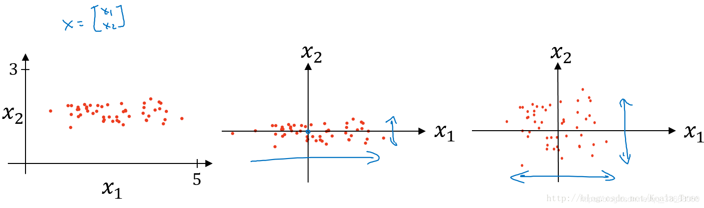在这里插入图片描述图中：左图为原始数据集分布，右是经过归一化处理后的数据集的分布，中间是经过均值操作后的分布。

第一部分结束。。。后续进行第二部分。。。 2020.01.14

2 参数初始化

参数的初始化能够极大的影响梯度下降的速度，比如说：如果激活函数选用 Sigmoid 或 tanh ，当 W 和 b 的值选择过大时，则 Z = WX + b 的值较大，得到的梯度趋于激活函数曲线的两端，导致每次迭代参数更新时下降梯度较小，训练过程就会变得比较缓慢; 相反，当 W 和 b 的值选择较小时，则 Z = WX + b 的值较小，处在0附近，0点区域的梯度比较大，故参数更新较快，训练过程就会变得比较快。

此外， W 参数的值不能都为0或相同的值，这是因为，当所有的W = 0或相同，整个网络就隐含层就没有意义了。

目前多采用的以下3中参数初始化策略：
随机初始化：W = np.random.randn( $n^[l]$ , $n^[l-1]$ )*0.01
He 初始化：W = np.random.randn( $n^[l]$ , $n^[l-1]$ )*sqrt(2/ $n^[l-1]$ ) （该方法在激活函数为Relu时效果好）
Xavier 初始化： W = np.random.randn( $n^[l]$ , $n^[l-1]$ )*sqrt(1/ $n^[l-1]$ ]) （该方法在激活函数为Sigmoid or tanh 时效果好）
这里： $n^[l]$ 代表该曾的神经元的个数； $n^[l-1]$ 代表上层神经元的个数;

代码实现：

def initialize_parameters_zeros(layer_dims):
    parameters = {}
    L = len(layer_dims)
    for l in range(1, L):
        parameters["W"+str(l)] = np.zeros((layer_dims[l], layer_dims[l-1]))
        parameters["b"+str(l)] = np.zeros((layer_dims[l], 1))
    return parameters

def initialize_parameters_random(layer_dims):
    np.random.seed(3)
    parameters = {}
    L = len(layer_dims)
    for l in range(1, L):
        parameters["W"+str(l)] = np.random.randn(layer_dims[l], layer_dims[l-1])
        parameters["b"+str(l)] = np.zeros((layer_dims[l], 1))
    return parameters
    
def initialize_parameters_he(layer_dims):
    np.random.seed(3)
    parameters = {}
    L = len(layer_dims) -1
    for l in range(1, L+1):
        parameters["W"+str(l)] = np.random.randn(layer_dims[l], layer_dims[l-1])*np.sqrt(2.0/layer_dims[l-1])
        parameters["b"+str(l)] = np.zeros((layer_dims[l], 1))
    return parameters

0初始化：

layer_dims = [2,3,2]
parameters = initialize_parameters_zeros(layer_dims)
结果：
{'b2': array([[0.],
       [0.]]), 'b1': array([[0.],
       [0.],
       [0.]]), 'W1': array([[0., 0.],
       [0., 0.],
       [0., 0.]]), 'W2': array([[0., 0., 0.],
       [0., 0., 0.]])}

随机初始化：

layer_dims = [2,3,2]
parameters = initialize_parameters_random(layer_dims)
结果：
{'b2': array([[0.],
       [0.]]), 'b1': array([[0.],
       [0.],
       [0.]]), 'W1': array([[ 1.78862847,  0.43650985],
       [ 0.09649747, -1.8634927 ],
       [-0.2773882 , -0.35475898]]), 'W2': array([[-0.08274148, -0.62700068, -0.04381817],
       [-0.47721803, -1.31386475,  0.88462238]])}

He 初始化：

parameters = initialize_parameters_he(layer_dims)
print (parameters)
结果：
{'b2': array([[0.],
       [0.]]), 'b1': array([[0.],
       [0.],
       [0.]]), 'W1': array([[ 1.78862847,  0.43650985],
       [ 0.09649747, -1.8634927 ],
       [-0.2773882 , -0.35475898]]), 'W2': array([[-0.06755814, -0.51194391, -0.03577739],
       [-0.38964689, -1.07276608,  0.72229115]])}

第二部分结束。。。后续进行第三部分。。。 2020.01.15

@阿文@

发布了15 篇原创文章 · 获赞 5 · 访问量 4385

私信关注

深度学习基础学习-forward&backward（1-数据集的处理）（内附python源码）

深度学习基础学习-forward&backward（数据集的处理及几种参数初始化策略）（内附python源码）

本篇博客从对数据集的处理开始到如何优化参数更新，全面覆盖BP神经网络的基础知识，以如何搭建一个BP的步骤为基本骨架进行逐个学习，主要内容包括以下几个方面：

1. 数据集的分批处理及归一化处理;

2. 参数的初始化;

3. 正则化;

4. 参数更行中的优化;

5. 学习率的优化;

6. 整个BP网络的搭建。

分步详解：

1 数据集的分批处理及归一化处理

（1）数据集的分批处理

（2）数据集的归一化处理

2 参数初始化

猜你喜欢