【手把手机器学习入门到放弃】sklearn决策树及其调参完全指南

使用sklearn构建决策树，并调优

sklearn学习包里的tree模块实现的就是CART树，但目前不支持离散变量的输入。

from sklearn import tree
from sklearn.model_selection import train_test_split
import graphviz
from sklearn import metrics
import pandas as pd
import numpy as np
import matplotlib.pyplot as plt
import seaborn as sns

不调参进行训练

#直接读取上次SVM的notebook中加工好的数据
X=pd.read_csv("american_salary_feture.csv")
y=pd.read_csv("american_salary_label.csv",header=None)
X_train, X_test, y_train, y_test = train_test_split(X,y,random_state=24)
clf=tree.DecisionTreeClassifier(random_state=24)
clf = clf.fit(X_train, y_train)

clf.score(X_test,y_test)

0.8135364205871515

print("test:",metrics.f1_score(clf.predict(X_test),y_test))
print("train",metrics.f1_score(clf.predict(X_train),y_train))

test: 0.6277587052476704
train 0.9999142440614013

在不进行调参的情况下，这明显是一个过拟合的模型，在训练集上的表现明显优于测试集上的表现，这也就是决策树的一个缺陷。

下面我们通过一些技术手段，让这个决策树更加符合实际。

sklearn官方文档中的参数描述

• criterion : string, optional (default=”gini”)

  The function to measure the quality of a split. Supported criteria are “gini” for the Gini impurity and “entropy” for the information gain.

  选择 gini 或者 entropy 选择以gini或是信息熵作为信息增益的计算

• splitter : string, optional (default=”best”)

  The strategy used to choose the split at each node. Supported strategies are “best” to choose the best split and “random” to choose the best random split.

  将连续变量分箱的方式，best选择最佳分箱方式，random选择最佳的随机分箱方式

• max_depth : int or None, optional (default=None)

  The maximum depth of the tree. If None, then nodes are expanded until all leaves are pure or until all leaves contain less than min_samples_split samples.

  决策树深度，如果不设置，那么决策树会分裂到直到所有的叶子节点中只含有同一种样本或者叶子中的样本数小于min_samples_split参数

• min_samples_split : int, float, optional (default=2)

  The minimum number of samples required to split an internal node:

  If int, then consider min_samples_split as the minimum number.

  If float, then min_samples_split is a fraction and ceil(min_samples_split * n_samples) are the minimum number of samples for each split.

  Changed in version 0.18: Added float values for fractions.

  如果是整数，就是每个叶子节点需要进一步分裂的最少样本数，如果是小数，那么这个最少样本个数等于min_samples_split*样本总数。

• min_samples_leaf : int, float, optional (default=1)

  The minimum number of samples required to be at a leaf node. A split point at any depth will only be considered if it leaves at least min_samples_leaf training samples in each of the left and right branches. This may have the effect of smoothing the model, especially in regression.

  If int, then consider min_samples_leaf as the minimum number.

  If float, then min_samples_leaf is a fraction and ceil(min_samples_leaf * n_samples) are the minimum number of samples for each node.

  Changed in version 0.18: Added float values for fractions.

  如果是整数，就是每个叶子节点最少容纳的样本数，如果是小数，那么每个叶子节点最少容纳的个数等于min_samples_leaf*样本总数。如果某个分裂条件下分裂出得某个子树含有的样本数小于这个数字，那么不能进行分裂。

• min_weight_fraction_leaf : float, optional (default=0.)

  The minimum weighted fraction of the sum total of weights (of all the input samples) required to be at a leaf node. Samples have equal weight when sample_weight is not provided.

  叶子节点最少需要占据总样本的比重，如果样本比重没有提供的话，每个样本占有相同比重

• max_features : int, float, string or None, optional (default=None)

  The number of features to consider when looking for the best split:

  If int, then consider max_features features at each split.

  If float, then max_features is a fraction and int(max_features * n_features) features are considered at each split.

  If “auto”, then max_features=sqrt(n_features).

  If “sqrt”, then max_features=sqrt(n_features).

  If “log2”, then max_features=log2(n_features).

  If None, then max_features=n_features.

  Note: the search for a split does not stop until at least one valid partition of the node samples is found, even if it requires to effectively inspect more than max_features features.

  分裂时需要考虑的最多的特征数，如果是整数，那么分裂时就考虑这几个特征，如果是小数，则分裂时考虑的特征数=max_features*总特征数，如果是“auto”或者“sqrt”，考虑的特征数是总特征数的平方根，如果是“log2”，考虑的特征数是log2（总特征素），如果是None，考虑的特征数=总特征数。需要注意的是，如果在规定的考虑特征数之内无法找到满足分裂条件的特征，那么决策树会继续寻找特征，直到找到一个满足分裂条件的特征。

• random_state : int, RandomState instance or None, optional (default=None)

  If int, random_state is the seed used by the random number generator; If RandomState instance, random_state is the random number generator; If None, the random number generator is the RandomState instance used by np.random.

  随机数值，用于打乱，默认使用np.random

• max_leaf_nodes : int or None, optional (default=None)

  Grow a tree with max_leaf_nodes in best-first fashion. Best nodes are defined as relative reduction in impurity. If None then unlimited number of leaf nodes.

  规定最多的叶子个数，根据区分度从高到低选择叶子节点，如果不传入这个参数，则不限制叶子节点个数。

• min_impurity_decrease : float, optional (default=0.)

  A node will be split if this split induces a decrease of the impurity greater than or equal to this value.

  The weighted impurity decrease equation is the following:

  N_t / N * (impurity - N_t_R / N_t * right_impurity
  - N_t_L / N_t * left_impurity)

  where N is the total number of samples, N_t is the number of samples at the current node, N_t_L is the number of samples in the left child, and N_t_R is the number of samples in the right child.

  N, N_t, N_t_R and N_t_L all refer to the weighted sum, if sample_weight is passed.

  New in version 0.19.

  最低分裂不纯度，当分裂后的减少的不纯度大于等于这个值时，才进行分裂。不纯度的计算公式如上。

• min_impurity_split : float, (default=1e-7)

  Threshold for early stopping in tree growth. A node will split if its impurity is above the threshold, otherwise it is a leaf.

  Deprecated since version 0.19: min_impurity_split has been deprecated in favor of min_impurity_decrease in 0.19. The default value of min_impurity_split will change from 1e-7 to 0 in 0.23 and it will be removed in 0.25. Use min_impurity_decrease instead.

  最少分裂阀值，如果一个节点的不纯度大于这个值的时候才进行分裂。

• class_weight : dict, list of dicts, “balanced” or None, default=None

  Weights associated with classes in the form {class_label: weight}. If not given, all classes are supposed to have weight one. For multi-output problems, a list of dicts can be provided in the same order as the columns of y.

  Note that for multioutput (including multilabel) weights should be defined for each class of every column in its own dict. For example, for four-class multilabel classification weights should be [{0: 1, 1: 1}, {0: 1, 1: 5}, {0: 1, 1: 1}, {0: 1, 1: 1}] instead of [{1:1}, {2:5}, {3:1}, {4:1}].

  The “balanced” mode uses the values of y to automatically adjust weights inversely proportional to class frequencies in the input data as n_samples / (n_classes * np.bincount(y))

  For multi-output, the weights of each column of y will be multiplied.

  Note that these weights will be multiplied with sample_weight (passed through the fit method) if sample_weight is specified.

  类别权重，对每个类别设置权重，示例如上，如果标签是多列的，那么每一列的的权重将会被相乘，如果在fit方法中传入了样本权重字典，那么类别权重会和样本权重相乘。

• presort : bool, optional (default=False)

  Whether to presort the data to speed up the finding of best splits in fitting. For the default settings of a decision tree on large datasets, setting this to true may slow down the training process. When using either a smaller dataset or a restricted depth, this may speed up the training.

  预排序，可以用来加速，注意在默认配置情况下，在数据集较大的情况下，预排序会降低训练速度，而在小样本或者在限制深度的情况下，预排序可以加速训练过程。

sklearn官方文档中的决策树优化建议

在官方文档中有一些优化建议，原文如下：（大致翻译了一下）

• Decision trees tend to overfit on data with a large number of features. Getting the right ratio of samples to number of features is important, since a tree with few samples in high dimensional space is very likely to overfit.

  特征数与样本数的平衡，样本数过小容易过拟合

• Consider performing dimensionality reduction (PCA, ICA, or Feature selection) beforehand to give your tree a better chance of finding features that are discriminative.

  对特征进行降维，使用PCA，ICA之类的技术，更有可能找到有区分度的特征

• Understanding the decision tree structure will help in gaining more insights about how the decision tree makes predictions, which is important for understanding the important features in the data.

  了解决策树的结构有利于了解数据中的重要特征

• Visualise your tree as you are training by using the export function. Use max_depth=3 as an initial tree depth to get a feel for how the tree is fitting to your data, and then increase the depth.

  将树可视化，初始使用比较小的深度来查看决策树是否适合用于训练这个数据。然后再慢慢增加深度。

• Remember that the number of samples required to populate the tree doubles for each additional level the tree grows to. Use max_depth to control the size of the tree to prevent overfitting.

  每增加一层深度需要的样本数就需要翻倍，所以控制好树的深度，避免过拟合。

• Use min_samples_split or min_samples_leaf to ensure that multiple samples inform every decision in the tree, by controlling which splits will be considered. A very small number will usually mean the tree will overfit, whereas a large number will prevent the tree from learning the data. Try min_samples_leaf=5 as an initial value. If the sample size varies greatly, a float number can be used as percentage in these two parameters. While min_samples_split can create arbitrarily small leaves, min_samples_leaf guarantees that each leaf has a minimum size, avoiding low-variance, over-fit leaf nodes in regression problems. For classification with few classes, min_samples_leaf=1 is often the best choice.

  使用min_samples_split min_samples_leaf两个参数保证每个叶子节点都有多个样本，如果每个叶子中的样本数很少，往往说明决策树过拟合了。从min_samples_leaf=5开始尝试。对于类别较少的分类问题，min_samples_leaf=1往往是最好的选择。

• Balance your dataset before training to prevent the tree from being biased toward the classes that are dominant. Class balancing can be done by sampling an equal number of samples from each class, or preferably by normalizing the sum of the sample weights (sample_weight) for each class to the same value. Also note that weight-based pre-pruning criteria, such as min_weight_fraction_leaf, will then be less biased toward dominant classes than criteria that are not aware of the sample weights, like min_samples_leaf.

  对数据集进行平衡性调整，以免整个树被数据量很大的树支配，将每个类别的样本数调整成一样的，或者更好的，将每个类别的样本权重调整成一样的。这样，根据权重进行剪枝的方案，如min_weight_fraction_leaf，会更好的调整样本的平衡性，比min_samples_leaf这种对权重不敏感的方案要好。

• If the samples are weighted, it will be easier to optimize the tree structure using weight-based pre-pruning criterion such as min_weight_fraction_leaf, which ensure that leaf nodes contain at least a fraction of the overall sum of the sample weights.

  如果增加了样本权重，那么就要使用对样本权重敏感的剪枝方案，如min_weight_fraction_leaf

• All decision trees use np.float32 arrays internally. If training data is not in this format, a copy of the dataset will be made.

  所有决策树的内部的数据类型是np.float32,如果不是这个数据类型，那么决策树会复制一个数据集。（考虑内存，可以自己先把数据集的数据类型调整好）

• If the input matrix X is very sparse, it is recommended to convert to sparse csc_matrix before calling fit and sparse csr_matrix before calling predict. Training time can be orders of magnitude faster for a sparse matrix input compared to a dense matrix when features have zero values in most of the samples.

  对于有很多0值的稀疏样本，建议将输入转换成csc_matrix再进行训练，并将测试集转换成csr_matrix再进行预测。这样可以节省很多时间。

下面我们根据官方文档的建议进行调优

构建一个三层树

clf=tree.DecisionTreeClassifier(max_depth =3,random_state=24)
clf.fit(X_train,y_train)

DecisionTreeClassifier(class_weight=None, criterion='gini', max_depth=3,
                       max_features=None, max_leaf_nodes=None,
                       min_impurity_decrease=0.0, min_impurity_split=None,
                       min_samples_leaf=1, min_samples_split=2,
                       min_weight_fraction_leaf=0.0, presort=False,
                       random_state=24, splitter='best')

#可视化
feature_name = X_train.columns
class_name =['0','1']
dot_data = tree.export_graphviz(clf, out_file=None, 
                     feature_names=feature_name,  
                     class_names=class_name,  
                     filled=True, rounded=True,  
                     special_characters=True)  
graph = graphviz.Source(dot_data)  
graph 

#分数
clf.score(X_test,y_test)

0.8400687876182287

print("test:",metrics.f1_score(clf.predict(X_test),y_test))
print("train",metrics.f1_score(clf.predict(X_train),y_train))

test: 0.6134204275534441
train 0.6132760560499131

在急剧减少树的深度之后，我们过拟合的问题解决了，但仍有可能欠拟合

平衡样本

y_train[0].value_counts()

0    18589
1     5831
Name: 0, dtype: int64

# 构建样本权重
sample_weight = np.zeros(y_train.shape[0])
sample_weight[y_train[0]==0]=1
sample_weight[y_train[0]==1]=18589/5831

clf=tree.DecisionTreeClassifier(max_depth =3, random_state=24)
clf = clf.fit(X_train, y_train,sample_weight=sample_weight)
print(clf.score(X_test,y_test))

0.8161159562707284

print("test:",metrics.f1_score(clf.predict(X_test),y_test))
print("train",metrics.f1_score(clf.predict(X_train),y_train))

test: 0.6509675915131732
train 0.6576849489795917

平衡样本之后我们的f1指标得到了很好的提升，虽然准确率下降了，但这个模型应该更加适用于预测。

转换成稀疏矩阵加速训练

根据官方建议，我们的训练数据由于有大量的哑变量，也就是有大量的0存在，所以压缩成稀疏矩阵可以加速训练，我们验证一下

from scipy import sparse
sX_train = sparse.csc_matrix(X_train)

未压缩的情况

%%time
clf=tree.DecisionTreeClassifier(max_depth=30,random_state=24)
clf = clf.fit(X_train, y_train)

CPU times: user 314 ms, sys: 4.98 ms, total: 319 ms
Wall time: 319 ms

压缩后的情况

%%time
clf=tree.DecisionTreeClassifier(max_depth=30,random_state=24)
clf = clf.fit(sX_train, y_train)

CPU times: user 913 ms, sys: 3.73 ms, total: 917 ms
Wall time: 916 ms

好像还是压缩后更慢，可能数据集中的0还不够多所以我们放弃压缩

调整树的深度

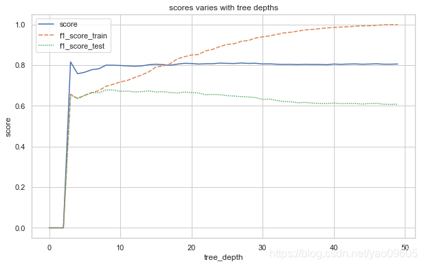
我们有20000多个样本，大概在2^14和215次方左右，我们取树的深度在10以内比较合适，不然是很容易过拟合的

depths = range(3,50)
score=np.zeros(50)
f1_score_train=np.zeros(50)
f1_score_test=np.zeros(50)
for depth in depths:
    clf=tree.DecisionTreeClassifier(max_depth =depth, random_state=24)
    clf.fit(X_train,y_train,sample_weight=sample_weight)
    score[depth]=clf.score(X_test,y_test)
    f1_score_test[depth] = metrics.f1_score(clf.predict(X_test), y_test)
    f1_score_train[depth] = metrics.f1_score(clf.predict(X_train), y_train)

plt.figure(figsize=(10,6))
sns.set(style="whitegrid")
data = pd.DataFrame({"score":score,"f1_score_train": f1_score_train,"f1_score_test": f1_score_test})
sns.lineplot(data=data)
plt.xlabel("tree_depth")
plt.ylabel("score")
plt.title("scores varies with tree depths")

Text(0.5, 1.0, 'scores varies with tree depths')

clf=tree.DecisionTreeClassifier(max_depth =8, random_state=24)
clf.fit(X_train,y_train,sample_weight=sample_weight)
print(clf.score(X_test,y_test))
print("test:",metrics.f1_score(clf.predict(X_test),y_test))
print("train",metrics.f1_score(clf.predict(X_train),y_train))

0.8000245670065103
test: 0.6781336496638987
train 0.6962163638847151

可以清楚看到随着树的深度的增加，测试集上与训练集上的表现差距越来越大，综合考虑三个指标，我们认为取max_depth=8是比较合适的一个数值

对 min_weight_fraction_leaf进行调参

由于我们的样本是带权重的，所以不适合使用min_samples_split，min_samples_leaf两个参数进行调参，如果样本本身比较平衡，那么可以使用这两个参数进行调参。

min_fractions = np.linspace(0,0.02,100,endpoint=True)
score_frac=np.zeros(100)
f1_score_test_frac=np.zeros(100)
f1_score_train_frac=np.zeros(100)
i=0
for min_fraction in min_fractions:
    clf=tree.DecisionTreeClassifier(max_depth =8, min_weight_fraction_leaf=min_fraction,random_state=24)
    clf.fit(X_train,y_train,sample_weight=sample_weight)
    score_frac[i]=clf.score(X_test,y_test)
    f1_score_test_frac[i] = metrics.f1_score(clf.predict(X_test), y_test)
    f1_score_train_frac[i] = metrics.f1_score(clf.predict(X_train), y_train)
    i=i+1

plt.figure(figsize=(10,6))
sns.set(style="whitegrid")
data = pd.DataFrame({"score":score_frac,"f1_score_train": f1_score_test_frac,"f1_score_test": f1_score_train_frac},
                   index=min_fractions)
sns.lineplot(data=data)
plt.xlabel("min_weight_fraction_leaf")
plt.ylabel("score")
plt.title("scores varies with min_weight_fraction_leaf")

Text(0.5, 1.0, 'scores varies with min_weight_fraction_leaf')

可以看到还是将这个权重设为0比较好，默认值也是0，就可以不用写了

PCA降维

为了把模型的训练加速，并且让树更简单在更少的层次中融入更多信息量，PCA是一个推荐的做法

from sklearn.decomposition import PCA

score_pca=np.zeros(30)
f1_score_test_pca=np.zeros(30)
f1_score_train_pca = np.zeros(30)
j=0
for i in range(1,31):
    pca=PCA(n_components=i,random_state=24)
    pca.fit(X_train)
    X_train_pca=pca.transform(X_train)
    X_test_pca=pca.transform(X_test)
    clf=tree.DecisionTreeClassifier(max_depth=8,random_state=24)
    clf.fit(X_train_pca,y_train,sample_weight=sample_weight)
    score_pca[j] = clf.score(X_test_pca,y_test)
    f1_score_test_pca[j]=metrics.f1_score(clf.predict(X_test_pca),y_test)
    f1_score_train_pca[j]=metrics.f1_score(clf.predict(X_train_pca),y_train)
    j=j+1

plt.figure(figsize=(10,6))
sns.set(style="whitegrid")
data = pd.DataFrame({"score":score_pca,"f1_score_train": f1_score_test_pca,"f1_score_test": f1_score_train_pca},
                   index=range(1,31))
sns.lineplot(data=data)
plt.xlabel("n_components")
plt.ylabel("score")
plt.title("scores varies with n_components")

Text(0.5, 1.0, 'scores varies with n_components')

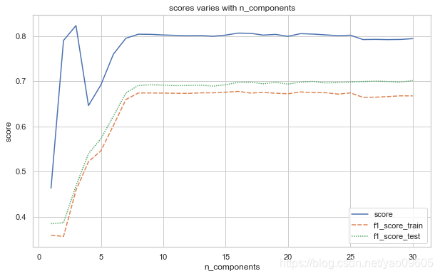
可以看到选择n_components值在8左右比较合适

pca=PCA(n_components=8,random_state=24)
pca.fit(X_train)
X_train_pca=pca.transform(X_train)
X_test_pca=pca.transform(X_test)
clf=tree.DecisionTreeClassifier(max_depth=8,random_state=24)
clf.fit(X_train_pca,y_train,sample_weight=sample_weight)
print(clf.score(X_test_pca,y_test))
print(metrics.f1_score(clf.predict(X_test_pca),y_test))
print(metrics.f1_score(clf.predict(X_train_pca),y_train))

0.8038324530156
0.6737487231869255
0.6905610284356879

可以看到在表现没有明显降低的情况下，我们的特征纬度降低到了8维。在训练和进行预测的时候速度都可以明显加快，同时也有缺点，就是可解释性变差。对于有些特征共线性比较小，那么PCA并不能降低太多的维度，那么做这个变化就没有必要了。

可视化树

clf=tree.DecisionTreeClassifier(max_depth =8, random_state=24)
clf.fit(X_train,y_train,sample_weight=sample_weight)
print(clf.score(X_test,y_test))
print("test:",metrics.f1_score(clf.predict(X_test),y_test))
print("train",metrics.f1_score(clf.predict(X_train),y_train))

0.8000245670065103
test: 0.6781336496638987
train 0.6962163638847151

#可视化
feature_name = np.array(X_train.columns)
for i in range(len(feature_name)):
    feature_name[i]=feature_name[i].replace("native-country","native_country")
    feature_name[i]=feature_name[i].replace("&","_")

class_name =['0','1']
dot_data = tree.export_graphviz(clf, out_file=None, 
                     feature_names=feature_name,  
                     class_names=class_name,  
                     filled=True, rounded=True,  
                     special_characters=True)  

type(feature_name[0])
feature_name[0]=feature_name[0].replace('a','e')
feature_name[0]

'ege'

graph = graphviz.Source(dot_data)  
graph 

图片

print("test:",metrics.classification_report(clf.predict(X_test),y_test))

test:               precision    recall  f1-score   support

           0       0.78      0.94      0.85      5093
           1       0.85      0.56      0.68      3048

    accuracy                           0.80      8141
   macro avg       0.82      0.75      0.77      8141
weighted avg       0.81      0.80      0.79      8141

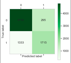
cm = metrics.confusion_matrix(y_test, clf.predict(X_test))
plt.matshow(cm,cmap=plt.cm.Greens)
plt.grid(False)
plt.colorbar()
for x in range(len(cm)):
    for y in range(len(cm)):
        plt.annotate(cm[x,y],xy=(x,y),horizontalalignment='center',verticalalignment='center')
plt.ylabel('True label')# 坐标轴标签

plt.xlabel('Predicted label')# 坐标轴标签

Text(0.5, 0, 'Predicted label')

总结

我们最后得到了一个比较平衡，且分类效果比较好的模型，我们使用了样本权重，调整深度，PCA三个方法来优化模型。
最后我们生成了决策树的图，可以看到结婚与否，工作时间，学历是影响收入比较重要的几个因素，结果也比较符合常识，预测准确率在80%左右。