cp8_Performance Python ( ipyparallel, sorted(list.items(),key=lambda k_v: (k_v[1], k_v[0]))

•如果某个应用对于效率非常敏感，那么一般来说应当检查两个方面：1）使用了正确的实现框架，2）使用了正确的效率库。在Python中可以使用很多种库来提升效率。本章将介绍如下的库：

•Cython，将Python与C框架结合起来进行静态编译

•Ipython.parallel，局部或在某个集群进行并行运算

•numexpr，快速数值计算

•multiprocessing, Python内建的处理（局部）并行运算的库

•Numba，为CPU动态编译Python代码

•NumbaPro，为CPU和GPU动态编译Python代码

Cython, for merging Python with C paradigms for static compilation
IPython.parallel, for the parallel execution of code/functions locally or over a
cluster
numexpr, for fast numerical operations
multiprocessing, Python’s built-in module for (local) parallel processing
Numba, for dynamically compiling Python code for the CPU
NumbaPro, for dynamically compiling Python code for multicore CPUs and GPUs

#per_comp_data(['f1'],['a_py'])
def per_comp_data(func_list, data_list, rep=3, number=1):
    from timeit import repeat
    res_list = {}
    print('function_list: ', func_list)
    for name in enumerate(func_list):
                         # f1                                #0
        stmt = name[1] + '(' + data_list[name[0]] + ')'
        setup = "from __main__ import " + name[1] + ', '+ data_list[name[0]]         #pre-process
        results = repeat(stmt=stmt, setup=setup, repeat=rep, number=number)
        res_list[name[1]] = sum(results) / rep   #function name :avg execute time or result

                                     #each ite                         #value or result  ,  # key or function name
    res_sort = sorted(res_list.items(),key=lambda k_v: (k_v[1], k_v[0]))
                                        #key=lambda (k, v): (v, k))
               
    for item in res_sort:

                 #each item's result  /   res_sort's first item's result           #relative    
        rel = item[1] / res_sort[0][1]
        print('function: '+ item[0] + ', av time sec: %9.5f, ' % item[1] + 'relative: %6.1f' % rel)

############################################################

############################################################

from math import *

def f(x):
    return abs(cos(x)) ** 0.5 + sin(2 + 3*x)

I = 500000
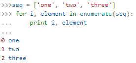
a_py = range(I)
a_py

#Standard Python function with explicit looping
def f1(a):
    res = []
    for x in a:
        res.append(f(x))
    return res

per_comp_data(['f1'],['a_py'])

#Iterator approach with implicit looping
def f2(a):
    return [f(x) for x in a]

eval

#Iterator approach with implicit looping and using eval
def f3(a):
    ex = 'abs(cos(x)) **0.5 + sin(2+3*x)'
    return [eval(ex) for x in a]

import numpy as np

a_np = np.arange(I)
a_np

#a_np = np.arange(I)
#NumPy vectorized implementation
def f4(a):                 #not a=range(I)                       #not a=range(I)
    return ( np.abs(np.cos( np.array(a) )) ** 0.5 + np.sin(2 +  3 * np.array(a)) )

Single-threaded implementation using numexpr

import numexpr as ne

#Single-threaded implementation using numexpr
def f5(a):
    ex = 'abs(cos(a)) **0.5 + sin(2+3*a)'
    ne.set_num_threads(1)
    return ne.evaluate(ex)

Multithreaded implementation using numexpr

#Multithreaded implementation using numexpr
def f6(a):
    ex = 'abs(cos(a)) **0.5 + sin(2+3*a)'
    ne.set_num_threads(16)
    return ne.evaluate(ex)

%%time
r1 = f1(a_py)
r2 = f2(a_py)
r3 = f3(a_py)
r4 = f4(a_py)
r5 = f5(a_py)
r6 = f6(a_py)

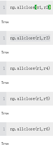
np.allclose(r1,r2)

func_list = ['f1', 'f2', 'f3', 'f4', 'f5', 'f6']
data_list = ['a_py', 'a_py', 'a_py', 'a_py', 'a_py', 'a_py']

per_comp_data(func_list, data_list)

import numpy as np

np.zeros( (3,3), dtype=np.float64, order='C')

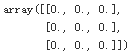
#C for C-like (i.e., row-wise)
#1, 2, and 3 are next to each other
c = np.array([[1.,1.,1,],
              [2.,2.,2.,],
              [3.,3.,3.]
             ], order='C')

#F for Fortran-like (i.e., column-wise)
f = np.array([[1.,1.,1,],
              [2.,2.,2.,],
              [3.,3.,3.]
             ], order='F')

x = np.random.standard_normal((3,1500000))
c = np.array(x, order='C')
f = np.array(x, order='F')
x = 0.0

Calculating sums over the first axis is roughly two times slower than over the second axis.

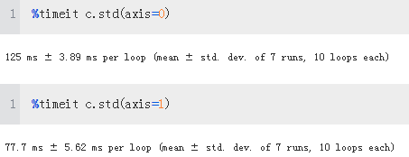
Again, this layout option leads to worse performance compared to the C-like layout. There is a small difference between the two axes, but again it is not as pronounced as with the other layout. The results indicate that in general the C-like option will perform better — which is also the reason why NumPy ndarray objects default to this memory layout if not otherwise specified:

https://blog.csdn.net/Linli522362242/article/details/90110433

def bsm_mcs_valuation(strike): #strike price of the option
    import numpy as np
    S0 =100
    T =1.0
    r=0.05        #riskless short rat
    vola=0.2
    
    M=50
    I=20000
    
    dt = T/M
    rand = np.random.standard_normal( (M+1, I) )
    S = np.zeros( (M+1, I) );
    S[0] = S0
    for t in range(1, M+1):                                         #np.random.standard_normal( (M+1, I) )
        S[t] = S[t-1] * np.exp( (r-0.5*vola**2)*dt + vola*np.sqrt(dt)*rand[t] )
        
    value = ( np.exp(-r * T)* np.sum( np.maximum(S[-1]-strike, 0) )/I )
    
    return value

def seq_value(n):
    strikes = np.linspace(80, 120, n)
    option_values = []
    for strike in strikes:
        option_values.append( bsm_mcs_valuation(strike) )
    return strikes, option_values

n = 100
%time strikes, option_values_seq = seq_value(n)

import matplotlib.pyplot as plt
%matplotlib inline

plt.figure( figsize=(8,4) )
plt.plot(strikes, option_values_seq, 'b') #curve
plt.plot(strikes, option_values_seq, 'r.')
plt.grid(True)
plt.xlabel('strikes')
plt.ylabel('European call option values')

#https://github.com/ipython/ipyparallel

from ipyparallel import Client
#from IPython import parallel
c = Client(profile='default')
view = c.load_balanced_view()

def par_value(n):
    strikes = np.linspace(80, 120, n)
    option_values = []
    for strike in strikes:
        value = view.apply_async(bsm_mcs_valuation, strike)
        option_values.append(value)
    c.wait(option_values)
    return strikes, option_values

%time strikes, option_values_obj = par_value(n)

option_values_obj[0].metadata

{'msg_id': 'd303c5cf-52d7809ddf9119e7013831bc',
 'submitted': datetime.datetime(2019, 7, 3, 22, 4, 26, 207524, tzinfo=tzutc()),
 'started': datetime.datetime(2019, 7, 3, 22, 4, 26, 301533, tzinfo=tzutc()),
 'completed': datetime.datetime(2019, 7, 3, 22, 4, 27, 391642, tzinfo=tzutc()),
 'received': datetime.datetime(2019, 7, 3, 22, 4, 28, 103714, tzinfo=tzutc()),
 'engine_uuid': 'aa607af7-40a54626e42be6d60d90677c',
 'engine_id': 7,
 'follow': [],
 'after': [],
 'status': 'ok',
 'execute_input': None,
 'execute_result': None,
 'error': None,
 'stdout': '',
 'stderr': '',
 'outputs': [],
 'data': {}}

option_values_obj[0].result()  #Note: we need the brackets

option_values_par = []
for res in option_values_obj:
    option_values_par.append(res.result())

option_values_par[:5]

plt.figure(figsize=(8,4))
plt.plot(strikes, option_values_seq, 'b', label='Sequential')
plt.plot(strikes, option_values_par, 'r.', label='Parallel')
plt.grid(True)
plt.legend(loc=0)
plt.xlabel('strikes')
plt.ylabel('European call option values')

Performance Comparison

n=50
func_list = ['seq_value', 'par_value']
data_list = 2*['n']

per_comp_data(func_list, data_list)

function_list:  ['seq_value', 'par_value']
function: par_value, av time sec:   3.77302, relative:    1.0
function: seq_value, av time sec:   5.12254, relative:    1.4

multiprocessing

The advantage of IPython.parallel is that it scales over small- and medium-sized clusters (e.g., with 256 nodes). Sometimes it is, however, helpful to parallelize code execution locally. This is where the “standard” multiprocessing module of Python might prove beneficial

•Ipython.parallel的优势是可以在中小规模群集（例如256个节点的群集）上伸缩。但是有时候 在本地并行执行代码是很有益的。这就是标准Python mulitprocessing模块的用武之地。我们用它处理几何布朗运动的模拟。

•首先，写一个几何布朗运动的模拟函数，这个函数返回以M和I为参数的模拟路径

•我们实现一个多核心处理中根据给定的参数值实现一个测试序列。假设我们需要进行100次模拟。

•结论是：性能和可用核心数量成正比，但是，超线程不能带来更多好处。

•金融学中许多问题可以应用简单的并行化技术，例如，在算法的不同实例之间没有共享数据时，Python的multiprocessing模块可以高效的利用现代硬件架构的能力，一般不需要改变基本算法或者并行执行的Python函数。