@article{cho2009kernel,
title={Kernel Methods for Deep Learning},
author={Cho, Youngmin and Saul, Lawrence K},
pages={342--350},
year={2009}}
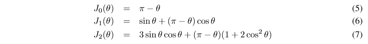
引
这篇文章介绍了一种新的核函数, 其启发来自于神经网络的运算.

其中\(\Theta(z)=\frac{1}{2}(1+\mathrm{sign}(z))\).
主要内容
主要性质, 公式(1)可以表示成:
\[ k_n(\mathbf{x}, \mathbf{y}) = \frac{1}{\pi} \|\mathbf{x}\|^n\|\mathbf{y}\|^n J_n(\theta). \tag{2} \]
其中:
\[ J_n(\theta) = (-1)^n (\sin \theta)^{2n+1} (\frac{1}{\sin \theta} \frac{\partial}{\partial \theta})^n(\frac{\pi-\theta}{\sin \theta}). \tag{3} \]
\[ \theta = \cos^{-1} (\frac{\mathbf{x}\cdot \mathbf{y}}{\|\mathbf{x}\| \|\mathbf{y}\|}). \tag{4} \]
特别的:
其证明如下:
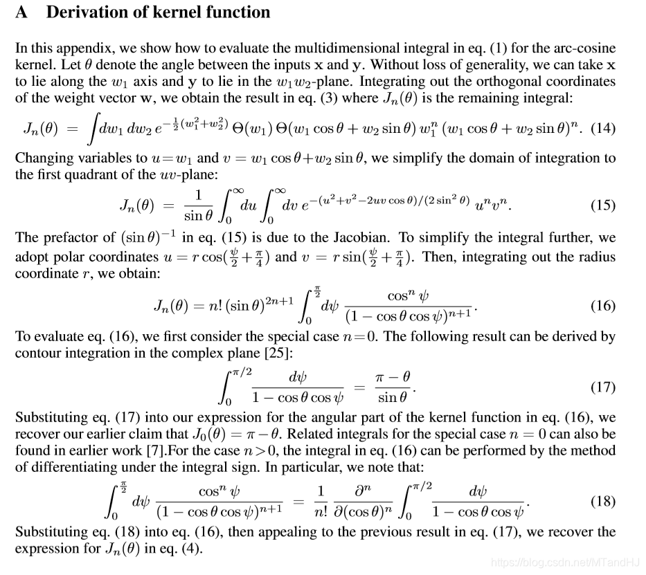
第(17)的证明我没有推, 因为 contour integration 暂时不了解.
细心的读者可能会发现, 最后的结果是\(\frac{\partial^n}{\partial(\cos \theta)^n}\), 注意对于一个函数\(f(\cos \theta)\), 我们可以令\(g(\theta) = f(\cos \theta)\)则:
\[ \frac{\partial f}{\partial \cos \theta} = \frac{\partial{g}}{\partial \theta} \frac{\partial\theta}{\partial \cos \theta}, \]
又
\[ \mathrm{d}\cos \theta =-\sin \theta \mathrm{d} \theta. \]
便得结论.
与深度学习的联系
如果我们把注意力集中在某一层, 假设输入为\(\mathbf{x}\), 输出为:
\[ \mathbf{f}(\mathbf{x}) = g(W\mathbf{x}) \in \mathbb{R}^m, \]
其中\(g(z) = \Theta(z) z^n\)是激活函数, 不同的n有如下的表现:
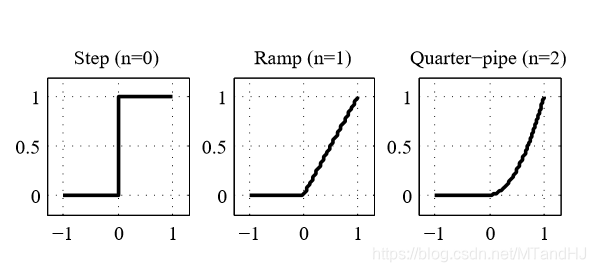
\(n=1\)便是我们熟悉的ReLU.
考虑俩个输入\(\mathbf{x},\mathbf{y}\)所对应的输出\(\mathbf{f}(\mathbf{x}),\mathbf{f}(\mathbf{y})\)的内积:
\[ \mathbf{f}(\mathbf{x}) \cdot \mathbf{f}(\mathbf{y}) = \sum_{i=1}^m \Theta(\mathbf{w}_i \cdot \mathbf{x}) \Theta(\mathbf{w}_i \cdot \mathbf{y}) (\mathbf{w}_i \cdot \mathbf{x})^n (\mathbf{w}_i \cdot \mathbf{y})^n \]
如果每个权重\(W_{ij}\)都服从标准正态分布, 则:
\[ \lim_{m \rightarrow \infty} \frac{2}{m} \mathbf{f} (\mathbf{x}) \cdot \mathbf{f}(\mathbf{x}) = k_n(\mathbf{x}, \mathbf{y}). \]
实验
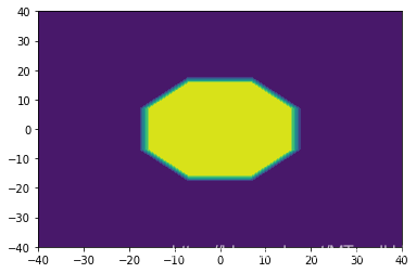
实验失败了, 代码如下.
import numpy as np
import pandas as pd
import matplotlib.pyplot as plt
from sklearn.svm import NuSVC
"""
Arc_cosine kernel
"""
class Arc_cosine:
def __init__(self, n=1):
self.n = n
self.own_kernel = self.kernels(n)
def kernel0(self, x, y):
norm_x = np.linalg.norm(x)
norm_y = np.linalg.norm(y)
cos_value = x @ y / (norm_x *
norm_y)
angle = np.arccos(cos_value)
return 1 - angle / np.pi
def kernel1(self, x, y):
norm_x = np.linalg.norm(x)
norm_y = np.linalg.norm(y)
cos_value = x @ y / (norm_x *
norm_y)
angle = np.arccos(cos_value)
sin_value = np.sin(angle)
return (norm_x * norm_y) ** self.n * \
(sin_value + (np.pi - angle) *
cos_value) / np.pi
def kernel2(self, x, y):
norm_x = np.linalg.norm(x)
norm_y = np.linalg.norm(y)
cos_value = x @ y / (norm_x *
norm_y)
angle = np.arccos(cos_value)
sin_value = np.sin(angle)
return (norm_x * norm_y) ** self.n * \
3 * sin_value * cos_value + \
(np.pi - angle) * (1 + 2 * cos_value ** 2)
def kernels(self, n):
if n is 0:
return self.kernel0
elif n is 1:
return self.kernel1
elif n is 2:
return self.kernel2
else:
raise ValueError("No such kernel, n should be "
"0, 1 or 2")
def kernel(self, X, Y):
m = X.shape[0]
n = Y.shape[0]
C = np.zeros((m, n))
for i in range(m):
for j in range(n):
C[i, j] = self.own_kernel(
X[i], Y[j]
)
return C
def __call__(self, X, Y):
return self.kernel(X, Y)
在俩个数据上进行SVM, 数据如下:
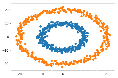
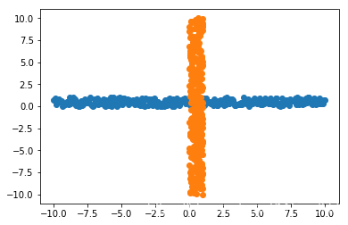
在SVM上跑:
'''
#生成圈圈数据
def generate_data(circle, r1, r2, nums=300):
    variance = 1
    rs1 = np.random.randn(nums) * variance + r1
    rs2 = np.random.randn(nums) * variance + r2
    angles = np.linspace(0, 2*np.pi, nums)
    data1 = (rs1 * np.sin(angles) + circle[0],
            rs1 * np.cos(angles) + circle[1])
    data2 = (rs2 * np.sin(angles) + circle[0],
            rs2 * np.cos(angles) + circle[1])
    df1 = pd.DataFrame({'x':data1[0], 'y': data1[1],
                        'label':np.ones(nums)})
    df2 = pd.DataFrame({'x':data2[0], 'y': data2[1],
                        'label':-np.ones(nums)})

    return df1, df2
'''

#生成十字数据
def generate_data(left, right, down, up,
                  circle=(0., 0.), nums=300):
    variance = 1
    y1 = np.random.rand(nums) * variance + circle[1]
    x2 = np.random.rand(nums) * variance + circle[0]
    x1 = np.linspace(left, right, nums)
    y2 = np.linspace(down, up, nums)
    df1 = pd.DataFrame(
        {'x': x1,
         'y': y1,
         'label':np.ones_like(x1)}
    )
    df2 = pd.DataFrame(
        {'x': x2,
         'y': y2,
         'label':-np.ones_like(x2)}
    )
    return df1, df2

def pre_test(left, right, func, nums=100):
    x1, y1 = left
    x2, y2 = right
    x = np.linspace(x1, x2, nums)
    y = np.linspace(y1, y2, nums)
    X,Y = np.meshgrid(x,y)
    m, n = X.shape
    Z = func(np.vstack((X.reshape(1, -1),
             Y.reshape(1, -1))).T).reshape(m, n)

    return X, Y, Z


df1, df2 = generate_data(-10, 10, -10, 10)
df = df1.append(df2)
classifer2 = NuSVC(kernel=Arc_cosine(n=1))
classifer2.fit(df.iloc[:, :2], df['label'])
X, Y, Z = pre_test((-10, -10), (10, 10), classifer2.predict)
plt.contourf(X, Y, Z)
plt.show()
预测结果均为:

而在一般的RBF上, 结果都是很好的:
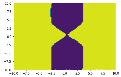
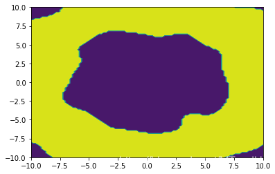
在多项式核上也ok:
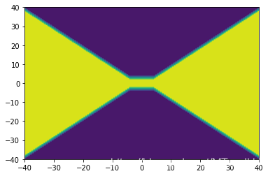
如果有人能发现代码中的错误,请务必指正.