1.np.repeat https://blog.csdn.net/u010496337/article/details/50572866/
import numpy as np
a=np.array(([1,2],[3,4]))
print(np.repeat(a,2))

#结果:
[1 1 2 2 3 3 4 4]
当axis=None时,会展平为一个行向量。
如果指定轴:
print(np.repeat(a,2,axis=0))

#结果
[[1 2]
 [1 2]
 [3 4]
 [3 4]]
2.DE工作。
如果是指定了两种细胞类型,那么就从两种cell类型中取样n_samples,当然是越多越好,经过VAE模型获取到了px_scales(经过校正)表达的百分比,之后用它计算贝贝叶斯因子,是通过判断两个矩阵的大小,并且求均值,log(res/1-res)。
如果是1 vs all,那么就轮流求,取样当前1的细胞类型的细胞,并将其他cell作为另一类,然后计算基因的贝叶斯因子。
3.对于np.random.choice函数
import numpy as np
print(np.random.choice([1,2,3,4],10))

#结果
[3 4 2 1 4 3 1 4 1 3]
如果要求的数目大于数组的长度,原来它是可以自动这样重复采样的啊。
4.去批分为两种,一种是同一个数据集中不同批次,另一种是多个数据集下的不同批次,比想象的复杂一点。
在调试时会出现此信息。
6.NearestNeighbors https://scikit-learn.org/stable/modules/generated/sklearn.neighbors.NearestNeighbors.html
#还是查文档好,接着就能看实现源码。
7.这个计算熵的可是真难理解:
        score += np.mean(
            [
                entropy(
                    batches[#Returns a tuple of arrays (row,col) containing the indices
                        kmatrix[indices].nonzero()[1][#找到权重不为0的
                            kmatrix[indices].nonzero()[0] == i
                        ]
                    ]
                )
                for i in range(n_samples_per_pool)#100
            ]
        )
终于明白了,举了个例子:
import numpy as np
km=np.array([[0,0,1],[1,0,0],[0,1,0]])
indices=[0,2]
print(km[indices].nonzero()[1][km[indices].nonzero()[0]==0])

#输出
[2]
>>> km[indices].nonzero()
(array([0, 1], dtype=int64), array([2, 1], dtype=int64))
>>> km[indices].nonzero()[0]==0
array([ True, False])
>>> km[indices].nonzero()[1]
array([2, 1], dtype=int64)
8.使用交叉熵函数:
![]()
当fre趋向于0或者1时,即差不多都属于同一批次的时候,熵就趋向于0。
9.再学习一下交叉熵。
https://blog.csdn.net/tsyccnh/article/details/79163834(待看)
10.tf.onehot,原始和类别,根据类别数据转换为onehot类型的。
https://blog.csdn.net/nini_coded/article/details/79250600
import tensorflow as tf

classes = 3
labels = tf.constant([0,1,2]) # 输入的元素值最小为0,最大为2
output = tf.one_hot(labels,classes)

sess = tf.Session()
with tf.Session() as sess:
    sess.run(tf.global_variables_initializer())
    output = sess.run(output)
    print("output of one-hot is : ",output)

# ('output of one-hot is : ',
# array([[ 1.,  0.,  0.],
#       [ 0.,  1.,  0.],
#       [ 0.,  0.,  1.]], dtype=float32))
并且手动尝试了一下:
import tensorflow as tf
a=tf.one_hot([0,0,0,1,1,1],2)
with tf.Session() as sess:
    print(sess.run(a))

#输出
[[1. 0.]
 [1. 0.]
 [1. 0.]
 [0. 1.]
 [0. 1.]
 [0. 1.]]
11.tf.random_normal https://blog.csdn.net/dcrmg/article/details/79028043
b= tf.random_normal([10])
with tf.Session() as sess:
    print(sess.run(b))

#输出
[-0.7680359   0.9331585   0.14169899  0.75573707 -1.3931639  -0.7400114
  0.58605003  1.8533127  -0.17746244 -1.0043402 ]
用于从服从指定正太分布的数值中取出指定个数的值。没有指定参数的话,就是标准正态分布。
12.没有激活函数的网络层?dense(h, self.n_input, activation=None)
https://cloud.tencent.com/developer/article/1061802(待看)
相当于f(x)=x。
13.tf.nn.softplus https://blog.csdn.net/ai_lx/article/details/88953587
import tensorflow as tf

a = tf.constant([-1.0, 12.0])
with tf.Session() as sess:
    b = tf.nn.softplus(a)
    print(sess.run(b))

#输出
[ 0.31326166 12.000006  ]
就是soft plus。#不是softmax,不是归一化。
公式是:log( exp( features ) + 1),所输入的a就是features。
14.搜索了ZINB的实现代码,未果,没有找到有类似的,
搜索 case_zero case_non_zero,找到了拟合ZINB分布的一个讲解,https://jdblischak.github.io/singlecell-qtl/zinb.html,看起来太复杂了。
就是说,计算ZINB似然的时候就是这么算的:
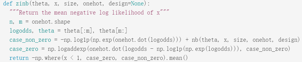
那么一般的似然值是如何计算的?似然值如何计算。
一般来说,给定参数θ以及服从的分布和原数据,就可以计算似然值,当前参数的似然值。但是现在我感觉好抽象,有没有个例子。