代码:
%% ------------------------------------------------------------------------
%% Output Info about this m-file
fprintf('\n***********************************************************\n');
fprintf(' <DSP using MATLAB> Problem 8.44.4 \n\n');
banner();
%% ------------------------------------------------------------------------
%%
%% Chebyshev-1 bandpass and highpass, parallel form,
%% by MATLAB toolbox function
%%
%% ------------------------------------------------------------------------
%--------------------------------------------------------
% PART1 bandpass
% Digital Filter Specifications: Chebyshev-1 bandpass
% -------------------------------------------------------
wsbp = [0.10*pi 0.60*pi]; % digital stopband freq in rad
wpbp = [0.20*pi 0.50*pi]; % digital passband freq in rad
delta1 = 0.1;
delta2 = 0.01;
Ripple = 1-delta1; % passband ripple in absolute
Attn = delta2; % stopband attenuation in absolute
Rp = -20*log10(Ripple); % passband ripple in dB
As = -20*log10(Attn); % stopband attenuation in dB
% Calculation of Chebyshev-1 filter parameters:
[N, wn] = cheb1ord(wpbp/pi, wsbp/pi, Rp, As);
fprintf('\n ********* Chebyshev-1 Digital Bandpass Filter Order is = %3.0f \n', 2*N)
% Digital Chebyshev-1 Bandpass Filter Design:
fprintf('\n*******Digital bandpass, Coefficients of DIRECT-form***********\n');
[bbp, abp] = cheby1(N, Rp, wn)
[C, B, A] = dir2cas(bbp, abp);
% Calculation of Frequency Response:
[dbbp, magbp, phabp, grdbp, wwbp] = freqz_m(bbp, abp);
% -----------------------------------------------------
% PART2 highpass
% Digital Highpass Filter Specifications:
% -----------------------------------------------------
wphp = 0.8*pi; % digital passband freq in rad
wshp = 0.7*pi; % digital stopband freq in rad
delta1 = 0.05;
delta2 = 0.01;
Ripple = 0.5-delta1; % passband ripple in absolute
Attn = delta2; % stopband attenuation in absolute
Rp = -20*log10(Ripple/0.5); % passband ripple in dB
As = -20*log10(Attn/0.5); % stopband attenuation in dB
% Calculation of Chebyshev-1 hp filter parameters:
[N, wn] = cheb1ord(wphp/pi, wshp/pi, Rp, As);
fprintf('\n********** Chebyshev-1 Digital Highpass Filter Order = %3.0f \n', N)
% Digital Chebyshev-1 Highpass Filter Design:
fprintf('\n*******Digital Highpass, Coefficients of DIRECT-form***********\n');
[bhp, ahp] = cheby1(N, Rp, wn, 'high')
[C, B, A] = dir2cas(bhp*0.5, ahp);
% Calculation of Frequency Response:
[dbhp, maghp, phahp, grdhp, wwhp] = freqz_m(bhp*0.5, ahp);
% ---------------------------------------------
% PART3 parallel form of bp and hp
% ---------------------------------------------
abp;
bbp;
ahp;
bhp;
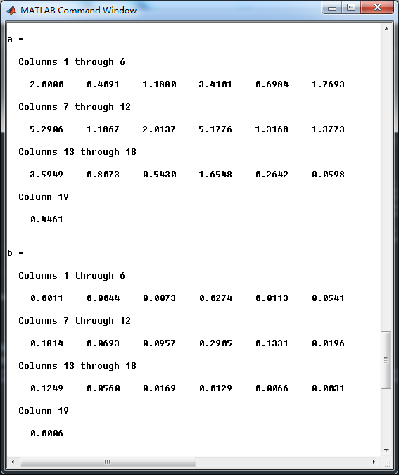
a = conv(2*abp, ahp)
b = conv(2*bbp, ahp) + conv(bhp, abp)
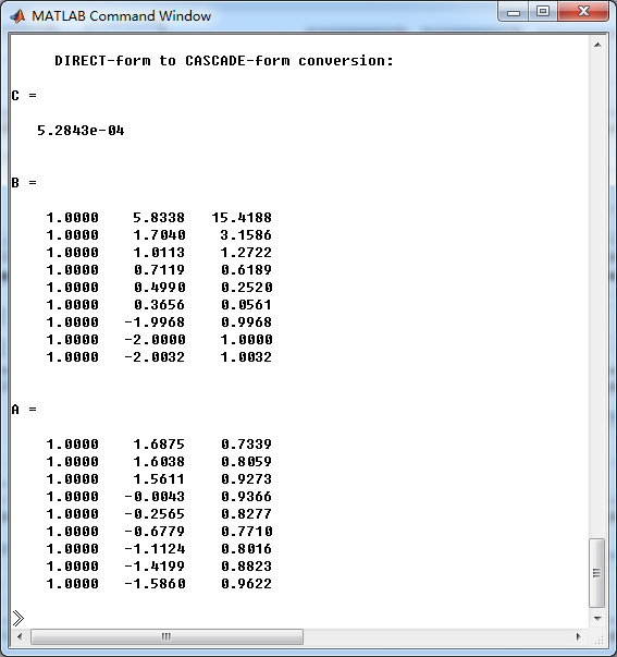
[C, B, A] = dir2cas(b, a)
% Calculation of Frequency Response:
[db, mag, pha, grd, ww] = freqz_m(b, a);
%% -----------------------------------------------------------------
%% Plot
%% -----------------------------------------------------------------
figure('NumberTitle', 'off', 'Name', 'Problem 8.44.4 combination of Chebyshev-1 bp and hp, by MATLAB cheby1 function')
set(gcf,'Color','white');
M = 1; % Omega max
subplot(2,2,1); plot(ww/pi, mag); axis([0, M, 0, 1.2]); grid on;
xlabel('Digital frequency in \pi units'); ylabel('|H|'); title('Magnitude Response');
set(gca, 'XTickMode', 'manual', 'XTick', [0, wsbp(1)/pi, wpbp/pi, wsbp(2)/pi, wshp/pi, wphp/pi, M]);
set(gca, 'YTickMode', 'manual', 'YTick', [0, 0.01, 0.45, 0.5, 0.9, 1]);
subplot(2,2,2); plot(ww/pi, db); axis([0, M, -100, 2]); grid on;
xlabel('Digital frequency in \pi units'); ylabel('Decibels'); title('Magnitude in dB');
set(gca, 'XTickMode', 'manual', 'XTick', [0, wsbp(1)/pi, wpbp/pi, wsbp(2)/pi, wshp/pi, wphp/pi, M]);
set(gca, 'YTickMode', 'manual', 'YTick', [-76, -46, -41, -1, 0]);
set(gca,'YTickLabelMode','manual','YTickLabel',['76'; '46'; '41';'1 ';' 0']);
subplot(2,2,3); plot(ww/pi, pha/pi); axis([0, M, -1.1, 1.1]); grid on;
xlabel('Digital frequency in \pi nuits'); ylabel('radians in \pi units'); title('Phase Response');
set(gca, 'XTickMode', 'manual', 'XTick', [0, wsbp(1)/pi, wpbp/pi, wsbp(2)/pi, wshp/pi, wphp/pi, M]);
set(gca, 'YTickMode', 'manual', 'YTick', [-1:0.5:1]);
subplot(2,2,4); plot(ww/pi, grd); axis([0, M, 0, 80]); grid on;
xlabel('Digital frequency in \pi units'); ylabel('Samples'); title('Group Delay');
set(gca, 'XTickMode', 'manual', 'XTick', [0, wsbp(1)/pi, wpbp/pi, wsbp(2)/pi, wshp/pi, wphp/pi, M]);
set(gca, 'YTickMode', 'manual', 'YTick', [0:20:80]);
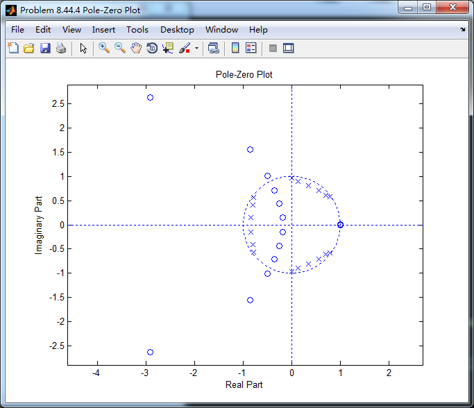
figure('NumberTitle', 'off', 'Name', 'Problem 8.44.4 Pole-Zero Plot')
set(gcf,'Color','white');
zplane(b, a);
title(sprintf('Pole-Zero Plot'));
%pzplotz(b,a);
figure('NumberTitle', 'off', 'Name', 'Problem 8.44.4 combination of Chebyshev-1 bp and hp, by MATLAB cheby1 function')
set(gcf,'Color','white');
M = 1; % Omega max
%subplot(2,2,1);
plot(ww/pi, mag); axis([0, M, 0, 1.2]); grid on;
xlabel('Digital frequency in \pi units'); ylabel('|H|'); title('Magnitude Response');
set(gca, 'XTickMode', 'manual', 'XTick', [0, wsbp(1)/pi, wpbp/pi, wsbp(2)/pi, wshp/pi, wphp/pi, M]);
set(gca, 'YTickMode', 'manual', 'YTick', [0, 0.01, 0.45, 0.5, 0.9, 1]);
运行结果:
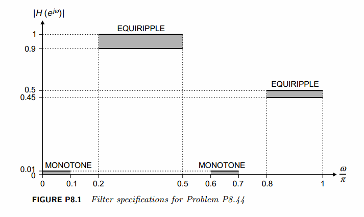
看设计要求,是Chebyshev-1型数字带通和高通滤波器的组合,首先计算带通。
系统函数直接形式系数如下:

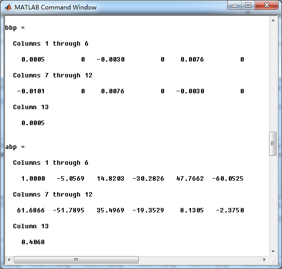
其次计算高通,系统函数直接形式系数如下:
再次,前面计算完高通和带通后,二者进行并联组合。等效滤波器的系统函数,直接形式系数如下:
串联形式的系数如下:
零极点图
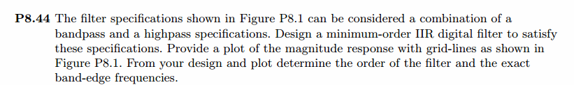
等效滤波器的幅度谱,相关幅度值、频带边界频率画出直线,如下图
