随着科研人员在使用神经网络训练时不断的尝试,为我们留下了很多有用的技巧,合理的运用这些技巧可以使自己的模型得到更好的拟合效果。
一 利用异或数据集演示过拟合
全连接网络虽然在拟合问题上比较强大,但太强大的拟合效果也带来了其它的麻烦,这就是过拟合问题。
首先我们看一个例子,这次将原有的4个异或带护具扩充成了上百个具有异或特征的数据集,然后通过全连接网络将它们进行分类。
实例描述:构建异或数据集模拟样本,在构建一个简单的多层神经网络来拟合其样本特征,观察其出现前泥河的现象,接着通过增大网络复杂性的方式来优化欠拟合问题,使其出现过拟合现象。
1. 构建异或数据集
'''
    生成随机数据
    '''
    np.random.seed(10)
    #特征个数
    num_features = 2
    #样本个数
    num_samples = 320
    #n返回长度为特征的数组 正太分布
    mean = np.random.randn(num_features)
    print('mean',mean)
    cov = np.eye(num_features)
    print('cov',cov)
    X,Y = generate(num_samples,mean,cov,[[3.0,0.0],[3.0,3.0],[0.0,3.0]],num_classes=4)
    #转换为二种类别
    Y = Y % 2

    xr = []
    xb = []

    for (l,k) in zip(Y[:],X[:]):
        if l == 0.0:
            xr.append([k[0],k[1]])
        else:
            xb.append([k[0],k[1]])

    xr = np.array(xr)
    xb = np.array(xb)
    plt.scatter(xr[:,0],xr[:,1],c='r',marker='+')
    plt.scatter(xb[:,0],xb[:,1],c='b',marker='o')

可以看到图上数据分为两类,左上和左下是一类,右上和右下是一类。
2 定义网络模型
'''
    定义变量
    '''
    #学习率
    learning_rate = 1e-4
    #输入层节点个数
    n_input = 2
    #隐藏层节点个数
    n_hidden = 2
    #输出节点数
    n_label = 1

    input_x = tf.placeholder(tf.float32,[None,n_input])
    input_y = tf.placeholder(tf.float32,[None,n_label])

    '''
    定义学习参数

    h1 代表隐藏层
    h2 代表输出层
    '''
    weights = {
            'h1':tf.Variable(tf.truncated_normal(shape=[n_input,n_hidden],stddev = 0.01)),     #方差0.1
            'h2':tf.Variable(tf.truncated_normal(shape=[n_hidden,n_label],stddev=0.01))
            }


    biases = {
            'h1':tf.Variable(tf.zeros([n_hidden])),
            'h2':tf.Variable(tf.zeros([n_label]))
            }


    '''
    定义网络模型
    '''
    #隐藏层
    layer_1 = tf.nn.relu(tf.add(tf.matmul(input_x,weights['h1']),biases['h1']))


    #代价函数
    y_pred = tf.nn.sigmoid(tf.add(tf.matmul(layer_1, weights['h2']),biases['h2']))
    loss = tf.reduce_mean(tf.square(y_pred - input_y))


    train = tf.train.AdamOptimizer(learning_rate).minimize(loss)
3. 训练网络并可视化显示
    '''
    开始训练
    '''
    training_epochs = 30000
    sess = tf.InteractiveSession()

    #初始化
    sess.run(tf.global_variables_initializer())

    for epoch in range(training_epochs):
        _,lo = sess.run([train,loss],feed_dict={input_x:X,input_y:np.reshape(Y,[-1,1])})
        if epoch % 1000 == 0:
            print('Epoch {0}  loss {1}'.format(epoch,lo))


    '''
    数据可视化
    '''
    nb_of_xs = 200
    xs1 = np.linspace(-1,8,num = nb_of_xs)
    xs2 = np.linspace(-1,8,num = nb_of_xs)

    #创建网格
    xx,yy = np.meshgrid(xs1,xs2)

    #初始化和填充 classfication plane
    classfication_plane = np.zeros([nb_of_xs,nb_of_xs])

    for i in range(nb_of_xs):
        for j in range(nb_of_xs):
            #计算每个输入样本对应的分类标签
            classfication_plane[i,j] = sess.run(y_pred,feed_dict={input_x:[[xx[i,j],yy[i,j]]]})

    #创建 color map用于显示
    cmap = ListedColormap([
                colorConverter.to_rgba('r',alpha = 0.30),
                colorConverter.to_rgba('b',alpha = 0.30),
            ])
    #显示各个样本边界
    plt.contourf(xx,yy,classfication_plane,cmap = cmap)
    plt.show()


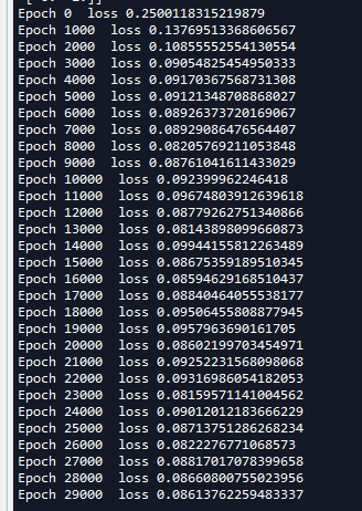
可以看到,模型在迭代训练20000次之后梯度更新就放缓了,而且loss值约等于16%并且准确率不高,所可视化的图片也没有将数据完全分开。
图上这种现象就叫做欠拟合,即没有完全拟合到想要得到的真实数据情况。
4 修正模型提高拟合度
欠拟合的原因并不是模型不行,而是我们的学习方法无法更精准地学习到适合的模型参数。模型越薄弱,对训练的要求就越高。但是可以采用增加节点或者增加层的方式,让模型具有更高的拟合性,从而降低模型的训练难度。
将隐藏层的节点个数改为200,代码如下:
    #隐藏层节点个数
    n_hidden = 200

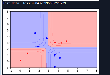
从图中可以看到强大的全连接网络,仅仅通过一个隐藏层,使用200个神经元就可以把数据划分的那么细致。而loss值也在逐渐变小,30000次之后已经变成了0.056.
5 验证过拟合
那么对于上面的模型好不好呢?我们再取少量的数据放到模型中验证一下,然后用同样的方式在坐标系中可视化。
'''
    测试  可以看到测试集loss值和训练集loss差距较大 这是因为模型过拟合了
    '''
    test_x,test_y = generate(12,mean,cov,[[3.0,0.0],[3.0,3.0],[0.0,3.0]],num_classes=4)
    #转换为二种类别
    test_y = test_y % 2


    xr = []
    xb = []

    for (l,k) in zip(test_y[:],test_x[:]):
        if l == 0.0:
            xr.append([k[0],k[1]])
        else:
            xb.append([k[0],k[1]])

    xr = np.array(xr)
    xb = np.array(xb)
    plt.figure()
    plt.scatter(xr[:,0],xr[:,1],c='r',marker='+')
    plt.scatter(xb[:,0],xb[:,1],c='b',marker='o')

    lo = sess.run(loss,feed_dict={input_x:test_x,input_y:np.reshape(test_y,[-1,1])})
    print('Test data  loss {0}'.format(lo))

    nb_of_xs = 200
    xs1 = np.linspace(-1,8,num = nb_of_xs)
    xs2 = np.linspace(-1,8,num = nb_of_xs)

    #创建网格
    xx,yy = np.meshgrid(xs1,xs2)

    #初始化和填充 classfication plane
    classfication_plane = np.zeros([nb_of_xs,nb_of_xs])

    for i in range(nb_of_xs):
        for j in range(nb_of_xs):
            #计算每个输入样本对应的分类标签
            classfication_plane[i,j] = sess.run(y_pred,feed_dict={input_x:[[xx[i,j],yy[i,j]]]})

    #创建 color map用于显示
    cmap = ListedColormap([
                colorConverter.to_rgba('r',alpha = 0.30),
                colorConverter.to_rgba('b',alpha = 0.30),
            ])
    #显示各个样本边界
    plt.contourf(xx,yy,classfication_plane,cmap = cmap)
    plt.show()

从这次运行结果,我们可以看到测试集的loss增加到了0.21,并没有原来训练时候的那么好0.056,模型还是原来的模型,但是这次却只框住了少量的样本。这种现象就是过拟合,它和欠拟合都是我们在训练模型中不愿意看到的现象,我们要的是真正的拟合在测试情况下能够变现出训练时的良好效果。
避免过拟合的方法有很多:常用的有early stopping、数据集扩展、正则化、弃权等,下面会使用这些方法来对该案例来进行优化。
6 通过正则化改善过拟合情况
Tensorflow中封装了L2正则化的函数可以直接使用:
tf.nn.l2_loss(t,name=None)
函数原型如下:
def l2_loss(t, name=None):
  r"""L2 Loss.

  Computes half the L2 norm of a tensor without the `sqrt`:

      output = sum(t ** 2) / 2

  Args:
    t: A `Tensor`. Must be one of the following types: `half`, `float32`, `float64`.
      Typically 2-D, but may have any dimensions.
    name: A name for the operation (optional).

  Returns:
    A `Tensor`. Has the same type as `t`. 0-D.
  """
  result = _op_def_lib.apply_op("L2Loss", t=t, name=name)
  return result
但是并没有提供L1正则化函数,但是可以自己组合:
tf.reduce_sum(tf.abs(w))
我们在代码中加入L2正则化:并设置返回参数lamda=1.6,修改代价函数如下:
loss = tf.reduce_mean(tf.square(y_pred - input_y)) + lamda * tf.nn.l2_loss(weights['h1'])/ num_samples + tf.nn.l2_loss(weights['h2']) *lamda/ num_samples


训练集的代价值从0.056增加到了0.106,但是测试集的代价值仅仅从0.21降到了0.0197,其效果并不是太明显。
7 通过增大数据集改善过拟合情况
下面再试试通过增大数据集的方法来改善过度拟合的情况,这里不再生产一个随机样本,而是每次从循环生成1000个数据。部分代码如下:
    for epoch in range(training_epochs):
        train_x,train_y = generate(num_samples,mean,cov,[[3.0,0.0],[3.0,3.0],[0.0,3.0]],num_classes=4)
        #转换为二种类别
        train_y = train_y % 2
        _,lo = sess.run([train,loss],feed_dict={input_x:train_x,input_y:np.reshape(train_y,[-1,1])})
        if epoch % 1000 == 0:
            print('Epoch {0}  loss {1}'.format(epoch,lo))
这次测试集代价值降到了0.04,比训练集还低,泛化效果更好了。
8 通过弃权改善过拟合情况
在TensorFlow中弃权的函数原型如下:
def dropout(x,keep_prob,noise_shape=None,seed=None,name=None)
其中的参数意义如下:
- x:输入的模型节点
- keep_prob:保存率,如果为1,则代表全部进行学习,如果为0.8,则代表丢弃20%的节点,只让80%的节点参与学习。
- noise_shape:指定x中,哪些维度可以使用dropout技术。
- seed:随机选择节点的过程中随机数的种子值。
dropout改变了神经网络的结构,它仅仅是属于训练时的方法,所以一般在进行测试时要将dropout的keep_prob设置为1,代表不需要进行丢弃,否则会影响模型的正常输出。
程序中加入了弃权,并且把keep_prob设置为0.5.
    '''
    定义网络模型
    '''
    #隐藏层
    layer_1 = tf.nn.relu(tf.add(tf.matmul(input_x,weights['h1']),biases['h1']))
    keep_prob = tf.placeholder(dtype=tf.float32)
    layer_1_drop = tf.nn.dropout(layer_1,keep_prob)

    #代价函数
    y_pred = tf.nn.sigmoid(tf.add(tf.matmul(layer_1_drop, weights['h2']),biases['h2']))
    loss = tf.reduce_mean(tf.square(y_pred - input_y))
输出结果如下,可以看到加入弃权改进也并不是多大,和L2正则化效果差不多。
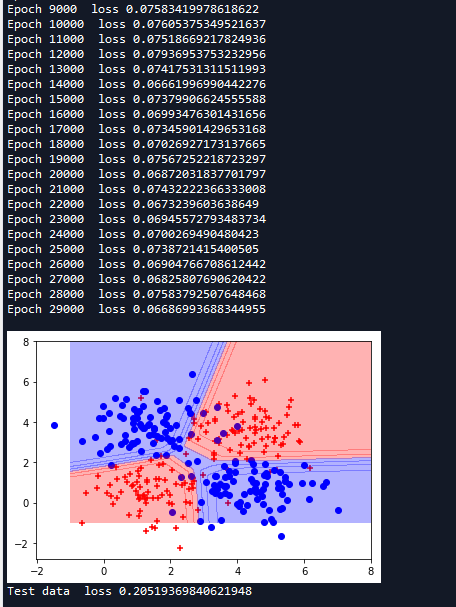
9 基于退化学习率dropout技术来拟合数据集
从上面结果可以看到代价值在来回波动,这主要是因为在训练后期出现了抖动现象,这表明学习率有点大了,这里我们可以添加退化学习率。
在使用优化器代码部分添加learning_rate,设置总步数为30000,每执行1000步,学习率衰减0.9,部分代码如下:
    '''
    定义网络模型
    '''
    #隐藏层
    layer_1 = tf.nn.relu(tf.add(tf.matmul(input_x,weights['h1']),biases['h1']))
    keep_prob = tf.placeholder(dtype=tf.float32)
    layer_1_drop = tf.nn.dropout(layer_1,keep_prob)

    #代价函数
    y_pred = tf.nn.sigmoid(tf.add(tf.matmul(layer_1_drop, weights['h2']),biases['h2']))
    loss = tf.reduce_mean(tf.square(y_pred - input_y))


    global_step = tf.Variable(0,trainable=False)
    decaylearning_rate = tf.train.exponential_decay(learning_rate,global_step,1000,0.9)
    train = tf.train.AdamOptimizer(decaylearning_rate).minimize(loss,global_step = global_step)


    '''
    开始训练
    '''
    training_epochs = 30000
    sess = tf.InteractiveSession()

    #初始化
    sess.run(tf.global_variables_initializer())

    for epoch in range(training_epochs):
        #执行一次train global_step变量会自加1
        rate,_,lo = sess.run([decaylearning_rate,train,loss],feed_dict={input_x:train_x,input_y:np.reshape(train_y,[-1,1]),keep_prob:0.5})
        if epoch % 1000 == 0:
            print('Epoch {0}   learning_rate  {1} loss {2} '.format(epoch,rate,lo))
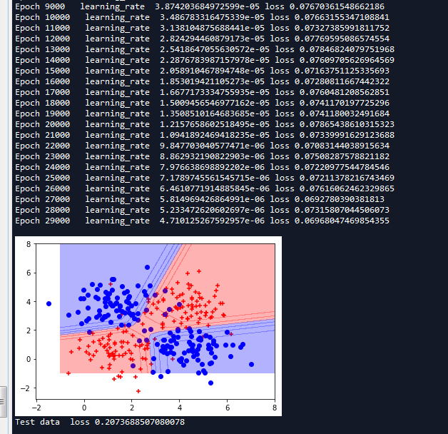
我们可以看到学习率是衰减了,但是效果并不是很明显,代价值还是在震荡,我们可以尝试调整一些参数,是的效果更好,这是一件需要耐心的事情。
完整代码:


# -*- coding: utf-8 -*-
"""
Created on Thu Apr 26 15:02:16 2018

@author: zy
"""

'''
通过一个过拟合的案例 来学习全网络训练中的优化技巧 比如:正则化,弃权等
'''

import  tensorflow  as tf
import  numpy as np
from sklearn.utils import shuffle
import matplotlib.pyplot as plt
import random
from matplotlib.colors import colorConverter, ListedColormap

'''
生成数据集
'''

def get_one_hot(labels,num_classes):
    '''
    one_hot编码

    args:
        labels : 输如类标签
        num_classes:类别个数
    '''
    m = np.zeros([labels.shape[0],num_classes])
    for i in range(labels.shape[0]):
        m[i][labels[i]] = 1
    return m


def  generate(sample_size,mean,cov,diff,num_classes=2,one_hot = False):
    '''
    因为没有医院的病例数据,所以模拟生成一些样本
    按照指定的均值和方差生成固定数量的样本

    args:
        sample_size:样本个数
        mean: 长度为 M 的 一维ndarray或者list  对应每个特征的均值
        cov: N X N的ndarray或者list  协方差  对称矩阵
        diff:长度为 类别-1 的list    每i元素为第i个类别和第0个类别均值的差值 [特征1差,特征2差....]  如果长度不够,后面每个元素值取diff最后一个元素
        num_classes:分类数
        one_hot : one_hot编码
    '''

    #每一类的样本数 假设有1000个样本 分两类,每类500个样本
    sample_per_class = int(sample_size/num_classes)


    '''
    多变量正态分布
    mean : 1-D array_like, of length N . Mean of the N-dimensional distribution.    数组类型,每一个元素对应一维的平均值
    cov : 2-D array_like, of shape (N, N) .Covariance matrix of the distribution. It must be symmetric and positive-semidefinite
        for proper sampling.
    size:shape. Given a shape of, for example, (m,n,k), m*n*k samples are generated, and packed in an m-by-n-by-k arrangement.
        Because each sample is N-dimensional, the output shape is (m,n,k,N). If no shape is specified, a single (N-D) sample is
        returned.
    '''
    #生成均值为mean,协方差为cov sample_per_class x len(mean)个样本 类别为0
    X0 = np.random.multivariate_normal(mean,cov,sample_per_class)
    Y0 = np.zeros(sample_per_class,dtype=np.int32)


    #对于diff长度不够进行处理
    if len(diff) != num_classes-1:
        tmp = np.zeros(num_classes-1)
        tmp[0:len(diff)] = diff
        tmp[len(diff):] = diff[-1]
    else:
        tmp = diff


    for ci,d  in enumerate(tmp):
        '''
        把list变成 索引-元素树,同时迭代索引和元素本身
        '''

        #生成均值为mean+d,协方差为cov sample_per_class x len(mean)个样本 类别为ci+1
        X1 = np.random.multivariate_normal(mean+d,cov,sample_per_class)
        Y1 = (ci+1)*np.ones(sample_per_class,dtype=np.int32)

        #合并X0,X1  按列拼接
        X0 = np.concatenate((X0,X1))
        Y0 = np.concatenate((Y0,Y1))


    if one_hot:
        Y0 = get_one_hot(Y0,num_classes)

    #打乱顺序
    X,Y  =  shuffle(X0,Y0)

    return X,Y


def example_overfit():
    '''
    显示一个过拟合的案例
    '''

    '''
    生成随机数据
    '''
    np.random.seed(10)
    #特征个数
    num_features = 2
    #样本个数
    num_samples = 320
    #n返回长度为特征的数组 正太分布
    mean = np.random.randn(num_features)
    print('mean',mean)
    cov = np.eye(num_features)
    print('cov',cov)
    train_x,train_y = generate(num_samples,mean,cov,[[3.0,0.0],[3.0,3.0],[0.0,3.0]],num_classes=4)
    #转换为二种类别
    train_y = train_y % 2


    xr = []
    xb = []

    for (l,k) in zip(train_y[:],train_x[:]):
        if l == 0.0:
            xr.append([k[0],k[1]])
        else:
            xb.append([k[0],k[1]])

    xr = np.array(xr)
    xb = np.array(xb)
    plt.scatter(xr[:,0],xr[:,1],c='r',marker='+')
    plt.scatter(xb[:,0],xb[:,1],c='b',marker='o')


    '''
    定义变量
    '''
    #学习率
    learning_rate = 1e-4
    #输入层节点个数
    n_input = 2
    #隐藏层节点个数
    n_hidden = 200   #设置为2则会欠拟合
    #输出节点数
    n_label = 1

    input_x = tf.placeholder(tf.float32,[None,n_input])
    input_y = tf.placeholder(tf.float32,[None,n_label])

    '''
    定义学习参数

    h1 代表隐藏层
    h2 代表输出层
    '''
    weights = {
            'h1':tf.Variable(tf.truncated_normal(shape=[n_input,n_hidden],stddev = 0.01)),     #方差0.1
            'h2':tf.Variable(tf.truncated_normal(shape=[n_hidden,n_label],stddev=0.01))
            }


    biases = {
            'h1':tf.Variable(tf.zeros([n_hidden])),
            'h2':tf.Variable(tf.zeros([n_label]))
            }


    '''
    定义网络模型
    '''
    #隐藏层
    layer_1 = tf.nn.relu(tf.add(tf.matmul(input_x,weights['h1']),biases['h1']))


    #代价函数
    y_pred = tf.nn.sigmoid(tf.add(tf.matmul(layer_1, weights['h2']),biases['h2']))
    loss = tf.reduce_mean(tf.square(y_pred - input_y))


    train = tf.train.AdamOptimizer(learning_rate).minimize(loss)


    '''
    开始训练
    '''
    training_epochs = 30000
    sess = tf.InteractiveSession()

    #初始化
    sess.run(tf.global_variables_initializer())

    for epoch in range(training_epochs):
        _,lo = sess.run([train,loss],feed_dict={input_x:train_x,input_y:np.reshape(train_y,[-1,1])})
        if epoch % 1000 == 0:
            print('Epoch {0}  loss {1}'.format(epoch,lo))


    '''
    数据可视化
    '''
    nb_of_xs = 200
    xs1 = np.linspace(-1,8,num = nb_of_xs)
    xs2 = np.linspace(-1,8,num = nb_of_xs)

    #创建网格
    xx,yy = np.meshgrid(xs1,xs2)

    #初始化和填充 classfication plane
    classfication_plane = np.zeros([nb_of_xs,nb_of_xs])

    for i in range(nb_of_xs):
        for j in range(nb_of_xs):
            #计算每个输入样本对应的分类标签
            classfication_plane[i,j] = sess.run(y_pred,feed_dict={input_x:[[xx[i,j],yy[i,j]]]})

    #创建 color map用于显示
    cmap = ListedColormap([
                colorConverter.to_rgba('r',alpha = 0.30),
                colorConverter.to_rgba('b',alpha = 0.30),
            ])
    #显示各个样本边界
    plt.contourf(xx,yy,classfication_plane,cmap = cmap)
    plt.show()


    '''
    测试  可以看到测试集loss值和训练集loss差距较大 这是因为模型过拟合了
    '''
    test_x,test_y = generate(12,mean,cov,[[3.0,0.0],[3.0,3.0],[0.0,3.0]],num_classes=4)
    #转换为二种类别
    test_y = test_y % 2


    xr = []
    xb = []

    for (l,k) in zip(test_y[:],test_x[:]):
        if l == 0.0:
            xr.append([k[0],k[1]])
        else:
            xb.append([k[0],k[1]])

    xr = np.array(xr)
    xb = np.array(xb)
    plt.figure()
    plt.scatter(xr[:,0],xr[:,1],c='r',marker='+')
    plt.scatter(xb[:,0],xb[:,1],c='b',marker='o')

    lo = sess.run(loss,feed_dict={input_x:test_x,input_y:np.reshape(test_y,[-1,1])})
    print('Test data  loss {0}'.format(lo))

    nb_of_xs = 200
    xs1 = np.linspace(-1,8,num = nb_of_xs)
    xs2 = np.linspace(-1,8,num = nb_of_xs)

    #创建网格
    xx,yy = np.meshgrid(xs1,xs2)

    #初始化和填充 classfication plane
    classfication_plane = np.zeros([nb_of_xs,nb_of_xs])

    for i in range(nb_of_xs):
        for j in range(nb_of_xs):
            #计算每个输入样本对应的分类标签
            classfication_plane[i,j] = sess.run(y_pred,feed_dict={input_x:[[xx[i,j],yy[i,j]]]})

    #创建 color map用于显示
    cmap = ListedColormap([
                colorConverter.to_rgba('r',alpha = 0.30),
                colorConverter.to_rgba('b',alpha = 0.30),
            ])
    #显示各个样本边界
    plt.contourf(xx,yy,classfication_plane,cmap = cmap)
    plt.show()


def example_l2_norm():
    '''
    显利用l2范数缓解过拟合
    '''

    '''
    生成随机数据
    '''
    np.random.seed(10)
    #特征个数
    num_features = 2
    #样本个数
    num_samples = 320
    #n返回长度为特征的数组 正太分布
    mean = np.random.randn(num_features)
    print('mean',mean)
    cov = np.eye(num_features)
    print('cov',cov)
    train_x,train_y = generate(num_samples,mean,cov,[[3.0,0.0],[3.0,3.0],[0.0,3.0]],num_classes=4)
    #转换为二种类别
    train_y = train_y % 2


    xr = []
    xb = []

    for (l,k) in zip(train_y[:],train_x[:]):
        if l == 0.0:
            xr.append([k[0],k[1]])
        else:
            xb.append([k[0],k[1]])

    xr = np.array(xr)
    xb = np.array(xb)
    plt.scatter(xr[:,0],xr[:,1],c='r',marker='+')
    plt.scatter(xb[:,0],xb[:,1],c='b',marker='o')


    '''
    定义变量
    '''
    #学习率
    learning_rate = 1e-4
    #输入层节点个数
    n_input = 2
    #隐藏层节点个数
    n_hidden = 200   #设置为2则会欠拟合
    #输出节点数
    n_label = 1
    #规范化参数
    lamda = 1.6

    input_x = tf.placeholder(tf.float32,[None,n_input])
    input_y = tf.placeholder(tf.float32,[None,n_label])

    '''
    定义学习参数

    h1 代表隐藏层
    h2 代表输出层
    '''
    weights = {
            'h1':tf.Variable(tf.truncated_normal(shape=[n_input,n_hidden],stddev = 0.01)),     #方差0.1
            'h2':tf.Variable(tf.truncated_normal(shape=[n_hidden,n_label],stddev=0.01))
            }


    biases = {
            'h1':tf.Variable(tf.zeros([n_hidden])),
            'h2':tf.Variable(tf.zeros([n_label]))
            }


    '''
    定义网络模型
    '''
    #隐藏层
    layer_1 = tf.nn.relu(tf.add(tf.matmul(input_x,weights['h1']),biases['h1']))


    #代价函数
    y_pred = tf.nn.sigmoid(tf.add(tf.matmul(layer_1, weights['h2']),biases['h2']))
    loss = tf.reduce_mean(tf.square(y_pred - input_y)) + lamda * tf.nn.l2_loss(weights['h1'])/ num_samples + tf.nn.l2_loss(weights['h2']) *lamda/ num_samples


    train = tf.train.AdamOptimizer(learning_rate).minimize(loss)


    '''
    开始训练
    '''
    training_epochs = 30000
    sess = tf.InteractiveSession()

    #初始化
    sess.run(tf.global_variables_initializer())

    for epoch in range(training_epochs):
        _,lo = sess.run([train,loss],feed_dict={input_x:train_x,input_y:np.reshape(train_y,[-1,1])})
        if epoch % 1000 == 0:
            print('Epoch {0}  loss {1}'.format(epoch,lo))


    '''
    数据可视化
    '''
    nb_of_xs = 200
    xs1 = np.linspace(-1,8,num = nb_of_xs)
    xs2 = np.linspace(-1,8,num = nb_of_xs)

    #创建网格
    xx,yy = np.meshgrid(xs1,xs2)

    #初始化和填充 classfication plane
    classfication_plane = np.zeros([nb_of_xs,nb_of_xs])

    for i in range(nb_of_xs):
        for j in range(nb_of_xs):
            #计算每个输入样本对应的分类标签
            classfication_plane[i,j] = sess.run(y_pred,feed_dict={input_x:[[xx[i,j],yy[i,j]]]})

    #创建 color map用于显示
    cmap = ListedColormap([
                colorConverter.to_rgba('r',alpha = 0.30),
                colorConverter.to_rgba('b',alpha = 0.30),
            ])
    #显示各个样本边界
    plt.contourf(xx,yy,classfication_plane,cmap = cmap)
    plt.show()


    '''
    测试  可以看到测试集loss值和训练集loss差距较大 这是因为模型过拟合了
    '''
    test_x,test_y = generate(12,mean,cov,[[3.0,0.0],[3.0,3.0],[0.0,3.0]],num_classes=4)
    #转换为二种类别
    test_y = test_y % 2


    xr = []
    xb = []

    for (l,k) in zip(test_y[:],test_x[:]):
        if l == 0.0:
            xr.append([k[0],k[1]])
        else:
            xb.append([k[0],k[1]])

    xr = np.array(xr)
    xb = np.array(xb)
    plt.figure()
    plt.scatter(xr[:,0],xr[:,1],c='r',marker='+')
    plt.scatter(xb[:,0],xb[:,1],c='b',marker='o')

    lo = sess.run(loss,feed_dict={input_x:test_x,input_y:np.reshape(test_y,[-1,1])})
    print('Test data  loss {0}'.format(lo))

    nb_of_xs = 200
    xs1 = np.linspace(-1,8,num = nb_of_xs)
    xs2 = np.linspace(-1,8,num = nb_of_xs)

    #创建网格
    xx,yy = np.meshgrid(xs1,xs2)

    #初始化和填充 classfication plane
    classfication_plane = np.zeros([nb_of_xs,nb_of_xs])

    for i in range(nb_of_xs):
        for j in range(nb_of_xs):
            #计算每个输入样本对应的分类标签
            classfication_plane[i,j] = sess.run(y_pred,feed_dict={input_x:[[xx[i,j],yy[i,j]]]})

    #创建 color map用于显示
    cmap = ListedColormap([
                colorConverter.to_rgba('r',alpha = 0.30),
                colorConverter.to_rgba('b',alpha = 0.30),
            ])
    #显示各个样本边界
    plt.contourf(xx,yy,classfication_plane,cmap = cmap)
    plt.show()


def example_add_trainset():
    '''
    通过增加训练集解过拟合
    '''

    '''
    生成随机数据
    '''
    np.random.seed(10)
    #特征个数
    num_features = 2
    #样本个数
    num_samples = 1000
    #n返回长度为特征的数组 正太分布
    mean = np.random.randn(num_features)
    print('mean',mean)
    cov = np.eye(num_features)
    print('cov',cov)


    '''
    定义变量
    '''
    #学习率
    learning_rate = 1e-4
    #输入层节点个数
    n_input = 2
    #隐藏层节点个数
    n_hidden = 200   #设置为2则会欠拟合
    #输出节点数
    n_label = 1


    input_x = tf.placeholder(tf.float32,[None,n_input])
    input_y = tf.placeholder(tf.float32,[None,n_label])

    '''
    定义学习参数

    h1 代表隐藏层
    h2 代表输出层
    '''
    weights = {
            'h1':tf.Variable(tf.truncated_normal(shape=[n_input,n_hidden],stddev = 0.01)),     #方差0.1
            'h2':tf.Variable(tf.truncated_normal(shape=[n_hidden,n_label],stddev=0.01))
            }


    biases = {
            'h1':tf.Variable(tf.zeros([n_hidden])),
            'h2':tf.Variable(tf.zeros([n_label]))
            }


    '''
    定义网络模型
    '''
    #隐藏层
    layer_1 = tf.nn.relu(tf.add(tf.matmul(input_x,weights['h1']),biases['h1']))


    #代价函数
    y_pred = tf.nn.sigmoid(tf.add(tf.matmul(layer_1, weights['h2']),biases['h2']))
    loss = tf.reduce_mean(tf.square(y_pred - input_y))


    train = tf.train.AdamOptimizer(learning_rate).minimize(loss)


    '''
    开始训练
    '''
    training_epochs = 30000
    sess = tf.InteractiveSession()

    #初始化
    sess.run(tf.global_variables_initializer())

    for epoch in range(training_epochs):
        train_x,train_y = generate(num_samples,mean,cov,[[3.0,0.0],[3.0,3.0],[0.0,3.0]],num_classes=4)
        #转换为二种类别
        train_y = train_y % 2
        _,lo = sess.run([train,loss],feed_dict={input_x:train_x,input_y:np.reshape(train_y,[-1,1])})
        if epoch % 1000 == 0:
            print('Epoch {0}  loss {1}'.format(epoch,lo))


    '''
    测试  可以看到测试集loss值和训练集loss差距较大 这是因为模型过拟合了
    '''
    test_x,test_y = generate(12,mean,cov,[[3.0,0.0],[3.0,3.0],[0.0,3.0]],num_classes=4)
    #转换为二种类别
    test_y = test_y % 2


    xr = []
    xb = []

    for (l,k) in zip(test_y[:],test_x[:]):
        if l == 0.0:
            xr.append([k[0],k[1]])
        else:
            xb.append([k[0],k[1]])

    xr = np.array(xr)
    xb = np.array(xb)
    plt.figure()
    plt.scatter(xr[:,0],xr[:,1],c='r',marker='+')
    plt.scatter(xb[:,0],xb[:,1],c='b',marker='o')

    lo = sess.run(loss,feed_dict={input_x:test_x,input_y:np.reshape(test_y,[-1,1])})
    print('Test data  loss {0}'.format(lo))

    nb_of_xs = 200
    xs1 = np.linspace(-1,8,num = nb_of_xs)
    xs2 = np.linspace(-1,8,num = nb_of_xs)

    #创建网格
    xx,yy = np.meshgrid(xs1,xs2)

    #初始化和填充 classfication plane
    classfication_plane = np.zeros([nb_of_xs,nb_of_xs])

    for i in range(nb_of_xs):
        for j in range(nb_of_xs):
            #计算每个输入样本对应的分类标签
            classfication_plane[i,j] = sess.run(y_pred,feed_dict={input_x:[[xx[i,j],yy[i,j]]]})

    #创建 color map用于显示
    cmap = ListedColormap([
                colorConverter.to_rgba('r',alpha = 0.30),
                colorConverter.to_rgba('b',alpha = 0.30),
            ])
    #显示各个样本边界
    plt.contourf(xx,yy,classfication_plane,cmap = cmap)
    plt.show()


def example_dropout():
    '''
    使用弃权解过拟合
    '''

    '''
    生成随机数据
    '''
    np.random.seed(10)
    #特征个数
    num_features = 2
    #样本个数
    num_samples = 320
    #n返回长度为特征的数组 正太分布
    mean = np.random.randn(num_features)
    print('mean',mean)
    cov = np.eye(num_features)
    print('cov',cov)
    train_x,train_y = generate(num_samples,mean,cov,[[3.0,0.0],[3.0,3.0],[0.0,3.0]],num_classes=4)
    #转换为二种类别
    train_y = train_y % 2


    xr = []
    xb = []

    for (l,k) in zip(train_y[:],train_x[:]):
        if l == 0.0:
            xr.append([k[0],k[1]])
        else:
            xb.append([k[0],k[1]])

    xr = np.array(xr)
    xb = np.array(xb)
    plt.scatter(xr[:,0],xr[:,1],c='r',marker='+')
    plt.scatter(xb[:,0],xb[:,1],c='b',marker='o')


    '''
    定义变量
    '''
    #学习率
    learning_rate = 1e-4
    #输入层节点个数
    n_input = 2
    #隐藏层节点个数
    n_hidden = 200   #设置为2则会欠拟合
    #输出节点数
    n_label = 1


    input_x = tf.placeholder(tf.float32,[None,n_input])
    input_y = tf.placeholder(tf.float32,[None,n_label])

    '''
    定义学习参数

    h1 代表隐藏层
    h2 代表输出层
    '''
    weights = {
            'h1':tf.Variable(tf.truncated_normal(shape=[n_input,n_hidden],stddev = 0.01)),     #方差0.1
            'h2':tf.Variable(tf.truncated_normal(shape=[n_hidden,n_label],stddev=0.01))
            }


    biases = {
            'h1':tf.Variable(tf.zeros([n_hidden])),
            'h2':tf.Variable(tf.zeros([n_label]))
            }


    '''
    定义网络模型
    '''
    #隐藏层
    layer_1 = tf.nn.relu(tf.add(tf.matmul(input_x,weights['h1']),biases['h1']))
    keep_prob = tf.placeholder(dtype=tf.float32)
    layer_1_drop = tf.nn.dropout(layer_1,keep_prob)

    #代价函数
    y_pred = tf.nn.sigmoid(tf.add(tf.matmul(layer_1_drop, weights['h2']),biases['h2']))
    loss = tf.reduce_mean(tf.square(y_pred - input_y))


    train = tf.train.AdamOptimizer(learning_rate).minimize(loss)


    '''
    开始训练
    '''
    training_epochs = 30000
    sess = tf.InteractiveSession()

    #初始化
    sess.run(tf.global_variables_initializer())

    for epoch in range(training_epochs):
        _,lo = sess.run([train,loss],feed_dict={input_x:train_x,input_y:np.reshape(train_y,[-1,1]),keep_prob:0.5})
        if epoch % 1000 == 0:
            print('Epoch {0}  loss {1}'.format(epoch,lo))


    '''
    数据可视化
    '''
    nb_of_xs = 200
    xs1 = np.linspace(-1,8,num = nb_of_xs)
    xs2 = np.linspace(-1,8,num = nb_of_xs)

    #创建网格
    xx,yy = np.meshgrid(xs1,xs2)

    #初始化和填充 classfication plane
    classfication_plane = np.zeros([nb_of_xs,nb_of_xs])

    for i in range(nb_of_xs):
        for j in range(nb_of_xs):
            #计算每个输入样本对应的分类标签
            classfication_plane[i,j] = sess.run(y_pred,feed_dict={input_x:[[xx[i,j],yy[i,j]]],keep_prob:1.0})

    #创建 color map用于显示
    cmap = ListedColormap([
                colorConverter.to_rgba('r',alpha = 0.30),
                colorConverter.to_rgba('b',alpha = 0.30),
            ])
    #显示各个样本边界
    plt.contourf(xx,yy,classfication_plane,cmap = cmap)
    plt.show()


    '''
    测试  可以看到测试集loss值和训练集loss差距较大 这是因为模型过拟合了
    '''
    test_x,test_y = generate(12,mean,cov,[[3.0,0.0],[3.0,3.0],[0.0,3.0]],num_classes=4)
    #转换为二种类别
    test_y = test_y % 2


    xr = []
    xb = []

    for (l,k) in zip(test_y[:],test_x[:]):
        if l == 0.0:
            xr.append([k[0],k[1]])
        else:
            xb.append([k[0],k[1]])

    xr = np.array(xr)
    xb = np.array(xb)
    plt.figure()
    plt.scatter(xr[:,0],xr[:,1],c='r',marker='+')
    plt.scatter(xb[:,0],xb[:,1],c='b',marker='o')

    lo = sess.run(loss,feed_dict={input_x:test_x,input_y:np.reshape(test_y,[-1,1]),keep_prob:1.0})
    print('Test data  loss {0}'.format(lo))

    nb_of_xs = 200
    xs1 = np.linspace(-1,8,num = nb_of_xs)
    xs2 = np.linspace(-1,8,num = nb_of_xs)

    #创建网格
    xx,yy = np.meshgrid(xs1,xs2)

    #初始化和填充 classfication plane
    classfication_plane = np.zeros([nb_of_xs,nb_of_xs])

    for i in range(nb_of_xs):
        for j in range(nb_of_xs):
            #计算每个输入样本对应的分类标签
            classfication_plane[i,j] = sess.run(y_pred,feed_dict={input_x:[[xx[i,j],yy[i,j]]],keep_prob:1.0})

    #创建 color map用于显示
    cmap = ListedColormap([
                colorConverter.to_rgba('r',alpha = 0.30),
                colorConverter.to_rgba('b',alpha = 0.30),
            ])
    #显示各个样本边界
    plt.contourf(xx,yy,classfication_plane,cmap = cmap)
    plt.show()


def example_dropout_learningrate_decay():
    '''
    使用弃权解过拟合 并使用退化学习率进行加速学习
    '''

    '''
    生成随机数据
    '''
    np.random.seed(10)
    #特征个数
    num_features = 2
    #样本个数
    num_samples = 320
    #n返回长度为特征的数组 正太分布
    mean = np.random.randn(num_features)
    print('mean',mean)
    cov = np.eye(num_features)
    print('cov',cov)
    train_x,train_y = generate(num_samples,mean,cov,[[3.0,0.0],[3.0,3.0],[0.0,3.0]],num_classes=4)
    #转换为二种类别
    train_y = train_y % 2


    xr = []
    xb = []

    for (l,k) in zip(train_y[:],train_x[:]):
        if l == 0.0:
            xr.append([k[0],k[1]])
        else:
            xb.append([k[0],k[1]])

    xr = np.array(xr)
    xb = np.array(xb)
    plt.scatter(xr[:,0],xr[:,1],c='r',marker='+')
    plt.scatter(xb[:,0],xb[:,1],c='b',marker='o')


    '''
    定义变量
    '''
    #学习率
    learning_rate = 1e-4
    #输入层节点个数
    n_input = 2
    #隐藏层节点个数
    n_hidden = 200   #设置为2则会欠拟合
    #输出节点数
    n_label = 1


    input_x = tf.placeholder(tf.float32,[None,n_input])
    input_y = tf.placeholder(tf.float32,[None,n_label])

    '''
    定义学习参数

    h1 代表隐藏层
    h2 代表输出层
    '''
    weights = {
            'h1':tf.Variable(tf.truncated_normal(shape=[n_input,n_hidden],stddev = 0.01)),     #方差0.1
            'h2':tf.Variable(tf.truncated_normal(shape=[n_hidden,n_label],stddev=0.01))
            }


    biases = {
            'h1':tf.Variable(tf.zeros([n_hidden])),
            'h2':tf.Variable(tf.zeros([n_label]))
            }


    '''
    定义网络模型
    '''
    #隐藏层
    layer_1 = tf.nn.relu(tf.add(tf.matmul(input_x,weights['h1']),biases['h1']))
    keep_prob = tf.placeholder(dtype=tf.float32)
    layer_1_drop = tf.nn.dropout(layer_1,keep_prob)

    #代价函数
    y_pred = tf.nn.sigmoid(tf.add(tf.matmul(layer_1_drop, weights['h2']),biases['h2']))
    loss = tf.reduce_mean(tf.square(y_pred - input_y))


    global_step = tf.Variable(0,trainable=False)
    decaylearning_rate = tf.train.exponential_decay(learning_rate,global_step,1000,0.9)
    train = tf.train.AdamOptimizer(decaylearning_rate).minimize(loss,global_step = global_step)


    '''
    开始训练
    '''
    training_epochs = 30000
    sess = tf.InteractiveSession()

    #初始化
    sess.run(tf.global_variables_initializer())

    for epoch in range(training_epochs):
        #执行一次train global_step变量会自加1
        rate,_,lo = sess.run([decaylearning_rate,train,loss],feed_dict={input_x:train_x,input_y:np.reshape(train_y,[-1,1]),keep_prob:0.5})
        if epoch % 1000 == 0:
            print('Epoch {0}   learning_rate  {1} loss {2} '.format(epoch,rate,lo))


    '''
    数据可视化
    '''
    nb_of_xs = 200
    xs1 = np.linspace(-1,8,num = nb_of_xs)
    xs2 = np.linspace(-1,8,num = nb_of_xs)

    #创建网格
    xx,yy = np.meshgrid(xs1,xs2)

    #初始化和填充 classfication plane
    classfication_plane = np.zeros([nb_of_xs,nb_of_xs])

    for i in range(nb_of_xs):
        for j in range(nb_of_xs):
            #计算每个输入样本对应的分类标签
            classfication_plane[i,j] = sess.run(y_pred,feed_dict={input_x:[[xx[i,j],yy[i,j]]],keep_prob:1.0})

    #创建 color map用于显示
    cmap = ListedColormap([
                colorConverter.to_rgba('r',alpha = 0.30),
                colorConverter.to_rgba('b',alpha = 0.30),
            ])
    #显示各个样本边界
    plt.contourf(xx,yy,classfication_plane,cmap = cmap)
    plt.show()


    '''
    测试  可以看到测试集loss值和训练集loss差距较大 这是因为模型过拟合了
    '''
    test_x,test_y = generate(12,mean,cov,[[3.0,0.0],[3.0,3.0],[0.0,3.0]],num_classes=4)
    #转换为二种类别
    test_y = test_y % 2


    xr = []
    xb = []

    for (l,k) in zip(test_y[:],test_x[:]):
        if l == 0.0:
            xr.append([k[0],k[1]])
        else:
            xb.append([k[0],k[1]])

    xr = np.array(xr)
    xb = np.array(xb)
    plt.figure()
    plt.scatter(xr[:,0],xr[:,1],c='r',marker='+')
    plt.scatter(xb[:,0],xb[:,1],c='b',marker='o')

    lo = sess.run(loss,feed_dict={input_x:test_x,input_y:np.reshape(test_y,[-1,1]),keep_prob:1.0})
    print('Test data  loss {0}'.format(lo))

    nb_of_xs = 200
    xs1 = np.linspace(-1,8,num = nb_of_xs)
    xs2 = np.linspace(-1,8,num = nb_of_xs)

    #创建网格
    xx,yy = np.meshgrid(xs1,xs2)

    #初始化和填充 classfication plane
    classfication_plane = np.zeros([nb_of_xs,nb_of_xs])

    for i in range(nb_of_xs):
        for j in range(nb_of_xs):
            #计算每个输入样本对应的分类标签
            classfication_plane[i,j] = sess.run(y_pred,feed_dict={input_x:[[xx[i,j],yy[i,j]]],keep_prob:1.0})

    #创建 color map用于显示
    cmap = ListedColormap([
                colorConverter.to_rgba('r',alpha = 0.30),
                colorConverter.to_rgba('b',alpha = 0.30),
            ])
    #显示各个样本边界
    plt.contourf(xx,yy,classfication_plane,cmap = cmap)
    plt.show()


if __name__== '__main__':
    #example_overfit()
    #example_l2_norm()
    #example_add_trainset()
    #example_dropout()
    example_dropout_learningrate_decay()