版权声明:本文为博主原创文章,遵循 CC 4.0 BY-SA 版权协议,转载请附上原文出处链接和本声明。
阅读扩展
TensorFlow 卷积神经网络
TensorFlow 循环神经网络
TensorFlow 序列预测
TensorFlow 官网示例
TensorFlow2.0❤️
基础运行示例
变量要经过初始化才能使用
import tensorflow as tf

# 创建tf格式的变量
a = tf.Variable([[1], [2]])
b = tf.Variable([[1, 2, 3]])
c = tf.matmul(a, b)

# 全局变量初始化
with tf.Session() as sess:
    init = tf.global_variables_initializer()
    sess.run(init)
    print(sess.run(c))
[[1 2 3]
[2 4 6]]
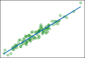
线性回归
from sklearn.datasets import make_regression
import tensorflow as tf, matplotlib.pyplot as mp

# 创建数据
x, y, coef = make_regression(n_features=1, noise=9, coef=True)
X = x.reshape(-1)

# 初始化W系数【shape=(1,),在[-1,1]的均匀分布中随机取值】
W = tf.Variable(tf.random_uniform([1], -1, 1))
# 初始化b系数【shape=(1,),值为0】
B = tf.Variable(tf.zeros([1]))
# 线性回归方程
Y = W * X + B

# 损失函数
loss = tf.reduce_mean(tf.square(Y - y))
# 梯度下降优化器,设置学习率
optimizer = tf.train.GradientDescentOptimizer(.3)
# 最小化损失
fit = optimizer.minimize(loss)

# 初始化全局变量
sess = tf.Session()
sess.run(tf.global_variables_initializer())

# 拟合
for step in range(10):
    print(' W:', sess.run(W), ' B:', sess.run(B),
          ' loss:', sess.run(loss), sep='')
    sess.run(fit)
w, b = sess.run(W)[0], sess.run(B)[0]
print('W=%f b=%f coef=%f' % (w, b, coef))

# 可视化
mp.scatter(x, y, c='g', alpha=.3)
mp.plot(x, w * x + b)
mp.show()
逻辑回归
from sklearn.datasets import make_blobs
import tensorflow as tf, matplotlib.pyplot as mp, numpy as np

# 创建随机样本
x, y = make_blobs(centers=2, cluster_std=3)
y = y.astype(np.float64).reshape(-1, 1)

# 系数初始化
W = tf.Variable(tf.random_normal([2, 1], dtype=tf.float64))
B = tf.Variable(tf.constant(.1, shape=[1], dtype=tf.float64))
H = tf.matmul(x, W) + B

# 损失函数
H = tf.nn.sigmoid(H)
loss = y * -tf.log(H) + (1 - y) * -tf.log(1 - H)
# loss = tf.nn.sigmoid_cross_entropy_with_logits(labels=y, logits=H)

# 梯度下降优化器,设置学习率,最小化损失
optimize = tf.train.AdamOptimizer(1e-1).minimize(loss)

# 运行
with tf.Session() as sess:
    sess.run(tf.global_variables_initializer())  # 全局变量初始化
    for step in range(99):
        print(sess.run(tf.reduce_mean(loss)))
        sess.run(optimize)  # 训练
    (w1, w2), b = sess.run(W), sess.run(B)

# 数据可视化
x1, x2 = x[:, 0], x[:, 1]
mp.scatter(x1, x2, c=y.reshape(-1))  # 原始样本点
x = np.array([x1.min(), x1.max()])
y = -(b + w1 * x) / w2  # 决策边界
mp.plot(x, y)
mp.show()

多层感知机
import tensorflow as tf
from tensorflow.examples.tutorials.mnist import input_data

"""配置"""
train_dir = 'data/'  # 数据集路径
units = 256  # 神经元数量

"""加载样本集:手写数字"""
mnist = input_data.read_data_sets(train_dir, one_hot=True)

"""多层感知机"""
# 输入层
X = tf.placeholder('float', [None, 28 * 28])
Y = tf.placeholder('float', [None, 10])  # 10分类(0~9)

# 全连接层1
W1 = tf.Variable(tf.truncated_normal([28 * 28, units], stddev=.1))
b1 = tf.Variable(tf.constant(.1, shape=[units]))
h1 = tf.nn.relu(tf.matmul(X, W1) + b1)

# 全连接层2
W2 = tf.Variable(tf.truncated_normal([units, 10], stddev=.1))
b2 = tf.Variable(tf.constant(.1, shape=[10]))
h2 = tf.matmul(h1, W2) + b2

# softmax交叉熵损失
loss = tf.nn.softmax_cross_entropy_with_logits(labels=Y, logits=h2)

# Adam优化器
optimizer = tf.train.AdamOptimizer().minimize(loss)

"""精度"""
prediction = tf.equal(tf.argmax(h2, 1), tf.argmax(Y, 1))
accuracy = tf.reduce_mean(tf.cast(prediction, 'float'))

"""运行"""
sess = tf.InteractiveSession()
sess.run(tf.global_variables_initializer())
batch_size = 50
for i in range(501):
    inputs, labels = mnist.train.next_batch(batch_size)  # 取一批
    optimizer.run(session=sess, feed_dict={X: inputs, Y: labels})  # 训练
    if i % 10 == 0:
        train_accuracy = accuracy.eval(session=sess, feed_dict={X: inputs, Y: labels})
        print('step %d, accuracy %g' % (i, train_accuracy))