数据平滑

数据平滑

数据的平滑处理通常包含有降噪、拟合等操作。降噪的功能意在去除额外的影响因素，拟合的目的意在数学模型化，可以通过更多的数学方法识别曲线特征。

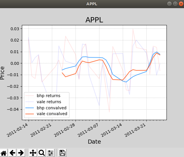
案例：绘制两只股票收益率曲线。收益率 =（后一天收盘价-前一天收盘价） / 前一天收盘价

 

　　使用卷积完成数据降噪。

# 数据平滑
import numpy as np
import matplotlib.pyplot as mp
import datetime as dt
import matplotlib.dates as md


def dmy2ymd(dmy):
  """
  把日月年转年月日
  :param day:
  :return:
  """
  dmy = str(dmy, encoding='utf-8')
  t = dt.datetime.strptime(dmy, '%d-%m-%Y')
  s = t.date().strftime('%Y-%m-%d')
  return s


dates, bhp_closing_prices = \
  np.loadtxt('bhp.csv',
             delimiter=',',
             usecols=(1, 6),
             unpack=True,
             dtype='M8[D],f8',
             converters={1: dmy2ymd})  # 日月年转年月日
vale_closing_prices = \
  np.loadtxt('vale.csv',
             delimiter=',',
             usecols=(6,),
             unpack=True)  # 因为日期一样,所以此处不读日期
# print(dates)
# 绘制收盘价的折现图
mp.figure('APPL', facecolor='lightgray')
mp.title('APPL', fontsize=18)
mp.xlabel('Date', fontsize=14)
mp.ylabel('Price', fontsize=14)
mp.grid(linestyle=":")

# 设置刻度定位器
# 每周一一个主刻度,一天一个次刻度

ax = mp.gca()
ma_loc = md.WeekdayLocator(byweekday=md.MO)
ax.xaxis.set_major_locator(ma_loc)
ax.xaxis.set_major_formatter(md.DateFormatter('%Y-%m-%d'))
ax.xaxis.set_minor_locator(md.DayLocator())
# 修改dates的dtype为md.datetime.datetiem
dates = dates.astype(md.datetime.datetime)

# 计算两只股票的收益率,并绘制曲线
bhp_returns = np.diff(bhp_closing_prices) / bhp_closing_prices[:-1]
vale_returns = np.diff(vale_closing_prices) / vale_closing_prices[:-1]
mp.plot(dates[1:], bhp_returns, color='red', alpha=0.1,label='bhp returns')
mp.plot(dates[1:], vale_returns, color='blue',alpha=0.1, label='vale returns')

#卷积降噪
kernel = np.hanning(8)
kernel/=kernel.sum()
bhp_convalved = np.convolve(bhp_returns,kernel,'valid')
vale_convalved = np.convolve(vale_returns,kernel,'valid')
mp.plot(dates[8:],bhp_convalved,color='dodgerblue',alpha=0.8,label='bhp convalved')
mp.plot(dates[8:],vale_convalved,color='orangered',alpha=0.8,label='vale convalved')

mp.legend()
mp.gcf().autofmt_xdate()
mp.show()

　　对处理过的股票收益率做多项式拟合。

# 数据平滑
import numpy as np
import matplotlib.pyplot as mp
import datetime as dt
import matplotlib.dates as md


def dmy2ymd(dmy):
  """
  把日月年转年月日
  :param day:
  :return:
  """
  dmy = str(dmy, encoding='utf-8')
  t = dt.datetime.strptime(dmy, '%d-%m-%Y')
  s = t.date().strftime('%Y-%m-%d')
  return s


dates, bhp_closing_prices = \
  np.loadtxt('bhp.csv',
             delimiter=',',
             usecols=(1, 6),
             unpack=True,
             dtype='M8[D],f8',
             converters={1: dmy2ymd})  # 日月年转年月日
vale_closing_prices = \
  np.loadtxt('vale.csv',
             delimiter=',',
             usecols=(6,),
             unpack=True)  # 因为日期一样,所以此处不读日期
# print(dates)
# 绘制收盘价的折现图
mp.figure('APPL', facecolor='lightgray')
mp.title('APPL', fontsize=18)
mp.xlabel('Date', fontsize=14)
mp.ylabel('Price', fontsize=14)
mp.grid(linestyle=":")

# 设置刻度定位器
# 每周一一个主刻度,一天一个次刻度

ax = mp.gca()
ma_loc = md.WeekdayLocator(byweekday=md.MO)
ax.xaxis.set_major_locator(ma_loc)
ax.xaxis.set_major_formatter(md.DateFormatter('%Y-%m-%d'))
ax.xaxis.set_minor_locator(md.DayLocator())
# 修改dates的dtype为md.datetime.datetiem
dates = dates.astype(md.datetime.datetime)

# 计算两只股票的收益率,并绘制曲线
bhp_returns = np.diff(bhp_closing_prices) / bhp_closing_prices[:-1]
vale_returns = np.diff(vale_closing_prices) / vale_closing_prices[:-1]
mp.plot(dates[1:], bhp_returns, color='red', alpha=0.1,label='bhp returns')
mp.plot(dates[1:], vale_returns, color='blue',alpha=0.1, label='vale returns')

#卷积降噪
kernel = np.hanning(8)
kernel/=kernel.sum()
bhp_convalved = np.convolve(bhp_returns,kernel,'valid')
vale_convalved = np.convolve(vale_returns,kernel,'valid')
mp.plot(dates[8:],bhp_convalved,color='dodgerblue',alpha=0.1,label='bhp convalved')
mp.plot(dates[8:],vale_convalved,color='orangered',alpha=0.1,label='vale convalved')

#多项式拟合
days = dates[8:].astype('M8[D]').astype('i4')
bhp_p = np.polyfit(days,bhp_convalved,3)
bhp_val = np.polyval(bhp_p,days)
vale_p = np.polyfit(days,vale_convalved,3)
vale_val = np.polyval(vale_p,days)
mp.plot(dates[8:],bhp_val,color='orangered',label='bhp polyval')
mp.plot(dates[8:],vale_val,color='blue',label='vale polyval')

mp.legend()
mp.gcf().autofmt_xdate()
mp.show()

　　通过获取两个函数的焦点可以分析两只股票的投资收益比。

# 数据平滑
import numpy as np
import matplotlib.pyplot as mp
import datetime as dt
import matplotlib.dates as md


def dmy2ymd(dmy):
  """
  把日月年转年月日
  :param day:
  :return:
  """
  dmy = str(dmy, encoding='utf-8')
  t = dt.datetime.strptime(dmy, '%d-%m-%Y')
  s = t.date().strftime('%Y-%m-%d')
  return s


dates, bhp_closing_prices = \
  np.loadtxt('bhp.csv',
             delimiter=',',
             usecols=(1, 6),
             unpack=True,
             dtype='M8[D],f8',
             converters={1: dmy2ymd})  # 日月年转年月日
vale_closing_prices = \
  np.loadtxt('vale.csv',
             delimiter=',',
             usecols=(6,),
             unpack=True)  # 因为日期一样,所以此处不读日期
# print(dates)
# 绘制收盘价的折现图
mp.figure('APPL', facecolor='lightgray')
mp.title('APPL', fontsize=18)
mp.xlabel('Date', fontsize=14)
mp.ylabel('Price', fontsize=14)
mp.grid(linestyle=":")

# 设置刻度定位器
# 每周一一个主刻度,一天一个次刻度

ax = mp.gca()
ma_loc = md.WeekdayLocator(byweekday=md.MO)
ax.xaxis.set_major_locator(ma_loc)
ax.xaxis.set_major_formatter(md.DateFormatter('%Y-%m-%d'))
ax.xaxis.set_minor_locator(md.DayLocator())
# 修改dates的dtype为md.datetime.datetiem
dates = dates.astype(md.datetime.datetime)

# 计算两只股票的收益率,并绘制曲线
bhp_returns = np.diff(bhp_closing_prices) / bhp_closing_prices[:-1]
vale_returns = np.diff(vale_closing_prices) / vale_closing_prices[:-1]
mp.plot(dates[1:], bhp_returns, color='red', alpha=0.1,label='bhp returns')
mp.plot(dates[1:], vale_returns, color='blue',alpha=0.1, label='vale returns')

#卷积降噪
kernel = np.hanning(8)
kernel/=kernel.sum()
bhp_convalved = np.convolve(bhp_returns,kernel,'valid')
vale_convalved = np.convolve(vale_returns,kernel,'valid')
mp.plot(dates[8:],bhp_convalved,color='dodgerblue',alpha=0.1,label='bhp convalved')
mp.plot(dates[8:],vale_convalved,color='orangered',alpha=0.1,label='vale convalved')

#多项式拟合
days = dates[8:].astype('M8[D]').astype('i4')

bhp_p = np.polyfit(days,bhp_convalved,3)
bhp_val = np.polyval(bhp_p,days)
vale_p = np.polyfit(days,vale_convalved,3)
vale_val = np.polyval(vale_p,days)
mp.plot(dates[8:],bhp_val,color='orangered',label='bhp polyval')
mp.plot(dates[8:],vale_val,color='blue',label='vale polyval')


#求两个多项式函数的焦点
diff_p = np.polysub(bhp_p,vale_p)
xs = np.roots(diff_p)
print(xs.astype('M8[D]'))
#['2011-03-23' '2011-03-11' '2011-02-21']


mp.legend()
mp.gcf().autofmt_xdate()
mp.show()