matplotlib---插值画二维、三维图

一、画二维图

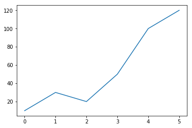
1.原始数据（x，y）

import matplotlib.pyplot as plt
import numpy as np

#数据
X = np.array(list(i for i in range(6)))
Y = np.array([10,30,20,50,100,120])

2.先对横坐标x进行扩充数据量，采用linspace

#插值
from scipy.interpolate import spline
X_new = np.linspace(X.min(),X.max(),300) #300 represents number of points to make between X.min and X.max

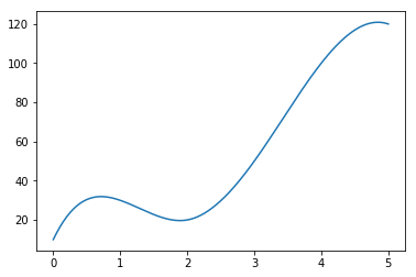
3.采用scipy.interpolate中的spline来对纵坐标数据y进行插值

由6个扩充到300个

smooth = spline(X,Y,X_new)

print(X_new.shape)  #（300，）
print(smooth.shape)  #（300，）

4.画图

#画图
plt.plot(X_new,smooth)
plt.show()

插值前	插值后

二、画三维图

1.载入数据

# 载入模块
import numpy as np
import matplotlib.pyplot as plt
from mpl_toolkits.mplot3d import Axes3D
from matplotlib import cm
import pandas as pd
import seaborn as sns
from scipy import interpolate

df_epsilon_alpha = pd.read_excel('实验记录_超参数.xlsx',sheet_name='epsilon_alpha')
#生成数据
epsilon = np.array(df_epsilon_alpha['epsilon'].values)
alpha = np.array(df_epsilon_alpha['alpha'].values)
Precision = np.array(df_epsilon_alpha['Precision'].values)

　　

2.将x和y扩充到想要的大小

【两种方法：np.arange和np.linspace】

xnew = np.arange(0.1, 1, 0.09) #左闭右闭每0.09间隔生成一个数
ynew = np.arange(0.1, 1, 0.09)  
或者

x = np.linspace(0.1,0.9,9)#0.1到0.9生成9个数
y = np.linspace(0.1,0.9,9)

　

3.对z插值

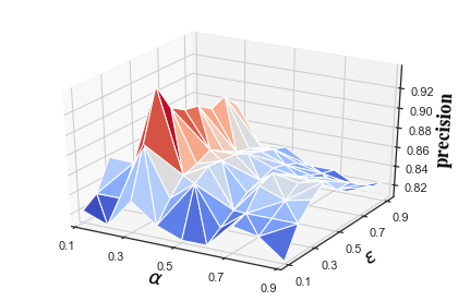
x,y原数据：

x = np.linspace(0.1,0.9,9)
y = np.linspace(0.1,0.9,9)
z = Precision

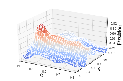
采用 scipy.interpolate.interp2d函数进行插值

f = interpolate.interp2d(x, y, z, kind='cubic')

x,y扩充数据：

xnew = np.arange(0.1, 1, 0.03)#(31,)
ynew = np.arange(0.1, 1, 0.03)#(31,)
znew = f(xnew, ynew)#(31,31) 

znew为插值后的z

4.画图

采用  from mpl_toolkits.mplot3d import Axes3D进行画三维图

Axes3D简单用法：

import matplotlib.pyplot as plt
from mpl_toolkits.mplot3d import Axes3D
fig = plt.figure()
ax = fig.add_subplot(111, projection='3d')

比如采用plot_trisurf画三维图：

plot_trisurf（x,y,z)

plot_trisurf对数据要求是：x.shape = y.shape = z.shape，所以x和y的shape需要修改，采用np.meshgrid，且都为一维数据

修改x,y,z输入画图函数前的shape

xx1, yy1 = np.meshgrid(xnew, ynew)#执行之后，xx1.shape=(31,31),yy1.shape=(31,31)
newshape = (xx1.shape[0])*(xx1.shape[0])
y_input = xx1.reshape(newshape)
x_input = yy1.reshape(newshape)
z_input = znew.reshape(newshape)

x_input.shape,y_input.shape,z_input.shape=((961,), (961,), (961,))

画图代码

#画图
sns.set(style='ticks')
fig = plt.figure()
ax = fig.add_subplot(111, projection='3d')
ax.plot_trisurf(x_input,y_input,z_input,cmap=cm.coolwarm)

plt.xlim((0.1,0.9))
plt.xticks([0.1,0.3,0.5,0.7,0.9])
plt.yticks([0.1,0.3,0.5,0.7,0.9])
ax.set_xlabel(r'$\alpha$',fontdict={'color': 'black',
                             'family': 'Times New Roman',
                             'weight': 'normal',
                             'size': 18})
ax.set_ylabel(r'$\epsilon$',fontdict={'color': 'black',
                             'family': 'Times New Roman',
                             'weight': 'normal',
                             'size': 18})
ax.set_zlabel('precision',fontdict={'color': 'black',
                             'family': 'Times New Roman',
                             'weight': 'normal',
                             'size': 18})

plt.tight_layout()
# plt.savefig('loc_svg/alpha_epsilon2.svg',dpi=600) #指定分辨率保存
plt.show()

插值前	插值后