数据统计分析中 y 和 x 的关系
- 线性关系:y = β * x
- 抛物线关系:y = β0 * x + β1 * x^2
- 对数关系:y = ln(x)
- 指数关系:y = e^x
- ...
主要内容
- 线性回归的模型、目标与算法
- 正则化方法:岭回归、LASSO算法、弹性网络
- 算法汇总:最小二乘法、极大似然估计、正则化的最小二乘法

扰动项就是不能被 X 解释的 Y 的变异,就是找不到解释的因素

简单线性回归的估计

import matplotlib.pyplot as plt
import os
import numpy as np
import pandas as pd
import statsmodels.api as sm
from statsmodels.formula.api import ols
os.chdir(r"D:\pydata")
#pd.set_option('display.max_columns', 8)
# 导入数据和数据清洗
# In[2]:
raw = pd.read_csv(r'creditcard_exp.csv', skipinitialspace=True)
raw.head()
# In[3]:
exp = raw[raw['avg_exp'].notnull()].copy().iloc[:, 2:].drop('age2',axis=1)
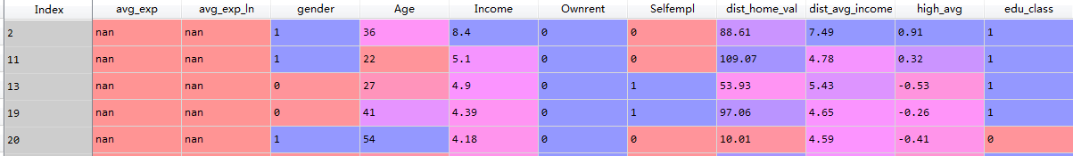
exp_new = raw[raw['avg_exp'].isnull()].copy().iloc[:, 2:].drop('age2',axis=1)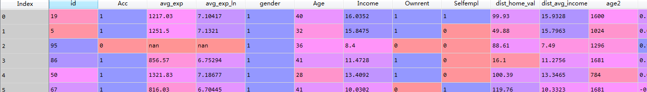
分出训练集和预测集

lm_s = ols('avg_exp ~ Income', data=exp).fit()
lm_s.summary()


                            OLS Regression Results
==============================================================================
Dep. Variable:                avg_exp   R-squared:                       0.454
Model:                            OLS   Adj. R-squared:                  0.446
Method:                 Least Squares   F-statistic:                     56.61
Date:                Fri, 26 Apr 2019   Prob (F-statistic):           1.60e-10
Time:                        14:10:26   Log-Likelihood:                -504.69
No. Observations:                  70   AIC:                             1013.
Df Residuals:                      68   BIC:                             1018.
Df Model:                           1
Covariance Type:            nonrobust
==============================================================================
                 coef    std err          t      P>|t|      [0.025      0.975]
------------------------------------------------------------------------------
Intercept    258.0495    104.290      2.474      0.016      49.942     466.157
Income        97.7286     12.989      7.524      0.000      71.809     123.648
==============================================================================
Omnibus:                        3.714   Durbin-Watson:                   1.424
Prob(Omnibus):                  0.156   Jarque-Bera (JB):                3.507
Skew:                           0.485   Prob(JB):                        0.173
Kurtosis:                       2.490   Cond. No.                         21.4
==============================================================================
Intercept 就是 β0,Income 就是 β1,y = 258.0495 + 97.7286 * x,这就分析出收入和支出的关系,但我们一般不关心截距 β0,因为可能没法解释(当收入为0时,支出为258.0495),我们关心斜率 β1,这个人的年收入每增加 1 万元,它的月均支出就增加97.7286 元。β1 的解释就是如何是连续变量, x 每增加一个单位,y 增减多少,如果是分类变量,则是有无 x,y 增减多少。但我们要先看 p 值,只有它显著,β1 才有意义,但我们不看 β0 的 p 值,如果不显著就把这个变量给删了,它在模型里没有意义,β0 无论显著不显著都带着
R-squared 描述模型优劣,模型解释力度,45.4%被解释了,越大越好,最大值为 1
Adj. R-squared,是选择模型用的,只有多个模型一起比较才有意义,AIC, BIC 也是如此(更倾向用)
模型评价-拟合优度

做预测
# Predict-在原始数据集上得到预测值和残差(实际值与预测值之差)

# In[8]:

pd.DataFrame([lm_s.predict(exp), lm_s.resid], index=['predict', 'resid']
            ).T.head()


Out[8]:
       predict       resid
0  1825.141904 -608.111904
1  1806.803136 -555.303136
3  1379.274813 -522.704813
4  1568.506658 -246.676658
5  1238.281793 -422.251793


lm_s.predict(exp_new)[:5]


Out[9]:
2     1078.969552
11     756.465245
13     736.919530
19     687.077955
20     666.554953
dtype: float64
多元线性回归


调整后的R2

多元回归例子

# ### 多元线性回归

# In[10]:

lm_m = ols('avg_exp ~ Age + Income + dist_home_val + dist_avg_income',
           data=exp).fit()
lm_m.summary()


                            OLS Regression Results
==============================================================================
Dep. Variable:                avg_exp   R-squared:                       0.542
Model:                            OLS   Adj. R-squared:                  0.513
Method:                 Least Squares   F-statistic:                     19.20
Date:                Fri, 26 Apr 2019   Prob (F-statistic):           1.82e-10
Time:                        15:36:20   Log-Likelihood:                -498.59
No. Observations:                  70   AIC:                             1007.
Df Residuals:                      65   BIC:                             1018.
Df Model:                           4
Covariance Type:            nonrobust
===================================================================================
                      coef    std err          t      P>|t|      [0.025      0.975]
-----------------------------------------------------------------------------------
Intercept         -32.0078    186.874     -0.171      0.865    -405.221     341.206
Age                 1.3723      5.605      0.245      0.807      -9.822      12.566
Income           -166.7204     87.607     -1.903      0.061    -341.684       8.243
dist_home_val       1.5329      1.057      1.450      0.152      -0.578       3.644
dist_avg_income   261.8827     87.807      2.982      0.004      86.521     437.245
==============================================================================
Omnibus:                        5.234   Durbin-Watson:                   1.582
Prob(Omnibus):                  0.073   Jarque-Bera (JB):                5.174
Skew:                           0.625   Prob(JB):                       0.0752
Kurtosis:                       2.540   Cond. No.                         459.
==============================================================================
发现 Age 和 dist_home_val 好像没什么作用,因为 p 值太大了,70个样本,α 选 0.1
由于多个变量 X 之间可能有相关性,可能会导致一些 X 提供的增量信息很少,变得不显著,所以要进行变量筛选,筛选无法提供增量信息的 X
多元线性回归的变量筛选

筛选方法

向前选择


# ### 多元线性回归的变量筛选

# In[11]: 向前回归法

'''forward select'''
def forward_select(data, response):
    remaining = set(data.columns)
    remaining.remove(response)
    selected = []
    current_score, best_new_score = float('inf'), float('inf')
    while remaining:
        aic_with_candidates=[]
        for candidate in remaining:
            formula = "{} ~ {}".format(
                response,' + '.join(selected + [candidate]))
            aic = ols(formula=formula, data=data).fit().aic
            aic_with_candidates.append((aic, candidate))
        aic_with_candidates.sort(reverse=True)
        best_new_score, best_candidate=aic_with_candidates.pop()
        if current_score > best_new_score:
            remaining.remove(best_candidate)
            selected.append(best_candidate)
            current_score = best_new_score
            print ('aic is {},continuing!'.format(current_score))
        else:
            print ('forward selection over!')
            break

    formula = "{} ~ {} ".format(response,' + '.join(selected))
    print('final formula is {}'.format(formula))
    model = ols(formula=formula, data=data).fit()
    return(model)


# In[12]:

data_for_select = exp[['avg_exp', 'Income', 'Age', 'dist_home_val',
                       'dist_avg_income']]
lm_m = forward_select(data=data_for_select, response='avg_exp')
print(lm_m.rsquared)


aic is 1007.6801413968115,continuing!
aic is 1005.4969816306302,continuing!
aic is 1005.2487355956046,continuing!
forward selection over!
final formula is avg_exp ~ dist_avg_income + Income + dist_home_val
0.541151292841195
可以看到通过 aic 筛选,并没有筛选去不显著的 dist_home_val
到后面其实我们可以先两两变量相关性检验,然后逐步法变量筛选,决策树或随机森林做模型筛选,再用 IV,最后再整个用逐步法再做一次。决策树做初筛行,但做细筛是不行的,因为他是根据变量覆盖的样本量来做的,不是说 X 对 Y 是否有影响这么做。