用keras进行猫狗识别（三）

版权声明：董瑞 https://blog.csdn.net/qq_39226755/article/details/89787768

背景

通过之前的数据增强+直接训练，我们将正确率提高到了八十以上，但是还有一种更好的方法去帮助我们训练，那就是使用预训练网络，原理就是前人栽树，后人乘凉，假定之前有人用了超多的数据进行训练，实现了多分类的识别，其中包括了我们本次要识别的东西，或者和我们识别的东西有相似特征的东西，这样我们就可以利用其训练的模型运用到自己的模型中。

首先介绍一下卷积神经网络，它主要包括两个部分，第一部分是卷积基，包括卷积层和池化层，第二个部分就是密集连接分类器，特征提取就是取出训练好的卷积基，在上边增加新的密集连接分类器，示意图如下：

准备文件

准备好训练集和验证集的图片，分别为2000张和1000张，倒是没有硬性要求，主要是为了学习，用的多就有点浪费时间了（原数据集有几万张）

进行预测数据，并保存

这个部分将用VGG16去训练我们的数据，指定没有分类器，最后我们将得到的数据进行储存，具体细节我写了注释，应该都能看懂

from keras.applications import VGG16

conv_base = VGG16(
    weights='imagenet',#指定模型初始化检查点
    include_top=False,#指定模型最后是否包含密集连接器
    input_shape=(150,150,3)#指定输入到网络中图像的形状
    )

import os
import numpy as np
from keras.preprocessing.image import ImageDataGenerator
#指定地址
base_dir = 'F:\DeepLearn\cat_and_dog'
train_dir = os.path.join(base_dir,'train')
test_dir = os.path.join(base_dir,'test')
validation_dir = os.path.join(base_dir,'check')

#配置图片生成器
datagen = ImageDataGenerator(rescale=1./255)
#设置批次
batch_size = 20

def extract_features(directory,sample_count):

    #本来是这样的，但是好像没什么大用，直接设置数组就行了
    #features = np.zeros(shape=(sample_count,4,4,512))
    #labels = np.zeros(shape=(sample_count))

    #设置两个数组，盛装特征和标签
    features=[]
    labels=[]

    #配置图片生成器,返回数组(x,y),x=(batchSize,targetSize,channels),y=标签
    generator = datagen.flow_from_directory(
        directory,
        target_size=(150,150),
        batch_size=batch_size,
        class_mode='binary'
    )
    i=0
    for input_batch,labels_batch in generator:
        #输入x：输入数据，输出预测数据
        features_batch = conv_base.predict(input_batch)
        features[i * batch_size : (i + 1) * batch_size] = features_batch
        labels[i * batch_size : (i + 1) * batch_size] = labels_batch
        i += 1
        if i * batch_size >= sample_count:
            break
    return features,labels

#得到预测数据
train_features, train_labels = extract_features(train_dir,2000)
validation_features, validation_labels = extract_features(validation_dir,1000)
test_features, test_labels = extract_features(test_dir,1000)

#将预测数据转化为二维形式
train_features = np.reshape(train_features,(2000,4*4*512))
validation_features = np.reshape(validation_features,(1000,4*4*512))
test_features = np.reshape(test_features,(1000,4*4*512))

#将预测数据储存
np.save('train_features.npy',train_features)
np.save('train_labels.npy',train_labels)
np.save('validation_features.npy',validation_features)
np.save('validation_labels.npy',validation_labels)
np.save('test_features.npy',test_features)
np.save('test_labels.npy',test_labels)

#将储存好的数据移动到一个文件夹中
if os.path.exists('./save_data/') == False:
    os.makedirs("./save_data/")
import shutil
f_list = os.listdir('./')
for f in f_list:
    if f.endswith('.npy'):
        if os.path.exists('./save_data/{0}'.format(f)) == True:
            os.remove('./save_data/{0}'.format(f))

预测结果

储存的文件形式如下

使用新的分类器

首先要取出我们训练的结果，然后创建一个新的分类器并进行训练，最后得到结果。

from keras import models
from keras import layers
from keras import optimizers
import numpy as np

#取出预测数据
train_features = np.load('./save_data/train_features.npy')
train_labels = np.load('./save_data/train_labels.npy')
validation_features = np.load('./save_data/validation_features.npy')
validation_labels = np.load('./save_data/validation_labels.npy')
test_features = np.load('./save_data/test_features.npy')
test_labels = np.load('./save_data/test_labels.npy')

#创建模型
model = models.Sequential()
model.add(layers.Dense(256,activation='relu',input_dim=4 * 4 * 512))
model.add(layers.Dropout(0.5))
model.add(layers.Dense(1,activation='sigmoid')) 

#设置优化器，损失函数，性能指标
model.compile(
    optimizer=optimizers.RMSprop(lr=2e-5),
    loss='binary_crossentropy',
    metrics=['acc']
)

#训练
history = model.fit(
    train_features,
    train_labels,
    epochs=30,
    batch_size=20,
    validation_data=(validation_features, validation_labels)
)

#画出结果，并储存
import matplotlib.pyplot as plt

acc = history.history['acc']
val_acc = history.history['val_acc']
loss = history.history['loss']
val_loss = history.history['val_loss']

epochs = range(1,len(acc) + 1)

plt.figure(1)
plt.plot(epochs,acc,'bo',label='Training acc')
plt.plot(epochs,val_acc,'b',label='Validation acc')
plt.title('Training and validation accuracy')
plt.legend()
plt.savefig('./save_data/preTrainAcc.png')
plt.show()

plt.figure(2)
plt.plot(epochs,loss,'bo',label='Training loss')
plt.plot(epochs,val_loss,'b',label='Validation loss')
plt.title('Training and validation loss')
plt.legend()
plt.savefig('./save_data/preTrainLoss.png')
plt.show()

得出训练结果

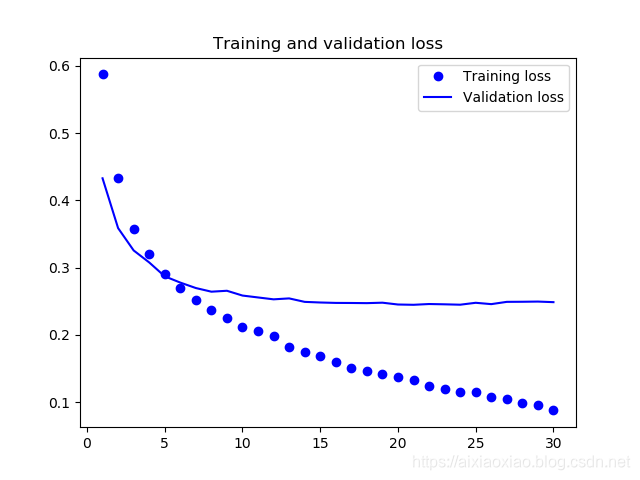
得出结论

从上边两张图可以看出，我们的准确度达到了88%到89%的这种感觉，比之前提高了不止一个档次，而且我觉得这种方法很方便，耗费的时间也比之前短，不过值得注意的是，在进行第十批次训练的时候就已经过拟合了，所以这个也需要用数据增强。