文章目录
- 1. 前馈神经网络、网络层数、输入层、隐藏层、输出层、隐藏单元、激活函数的概念。
- 2. 感知机相关;利用tensorflow等工具定义简单的几层网络(激活函数sigmoid),递归使用链式法则来实现反向传播。
- 3. 激活函数的种类以及各自的提出背景、优缺点。(和线性模型对比,线性模型的局限性,去线性化)
- 4. 深度学习中的正则化(参数范数惩罚:L1正则化、L2正则化;数据集增强;噪声添加;early stop;Dropout层)、正则化的介绍。
- 5. 深度模型中的优化:参数初始化策略;自适应学习率算法(梯度下降、AdaGrad、RMSProp、Adam;优化算法的选择);batch norm层(提出背景、解决什么问题、层在训练和测试阶段的计算公式);layer norm层。
1. 前馈神经网络、网络层数、输入层、隐藏层、输出层、隐藏单元、激活函数的概念。
1.1 前馈神经网络(feedforward neural network)
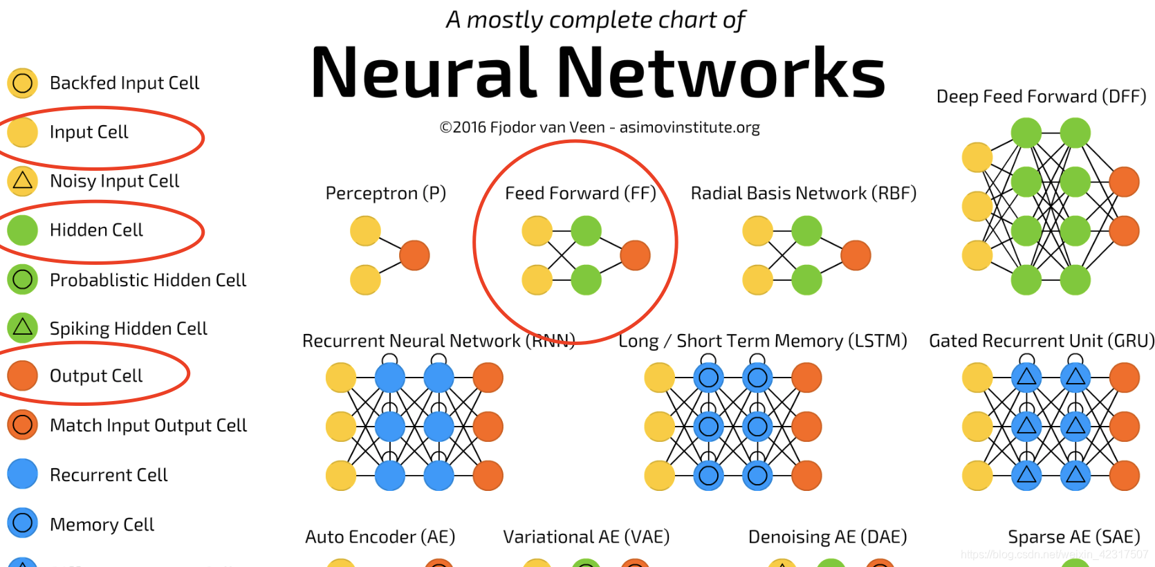
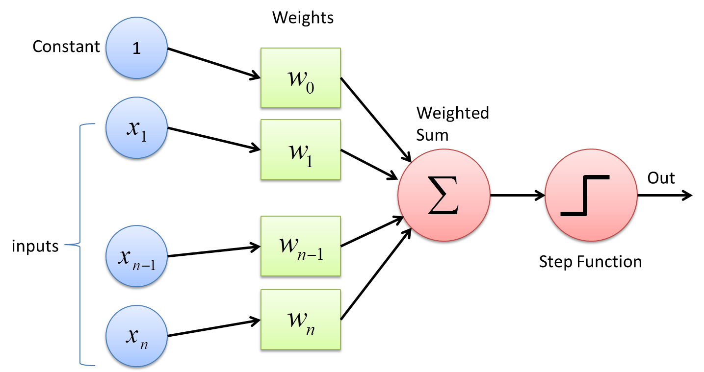
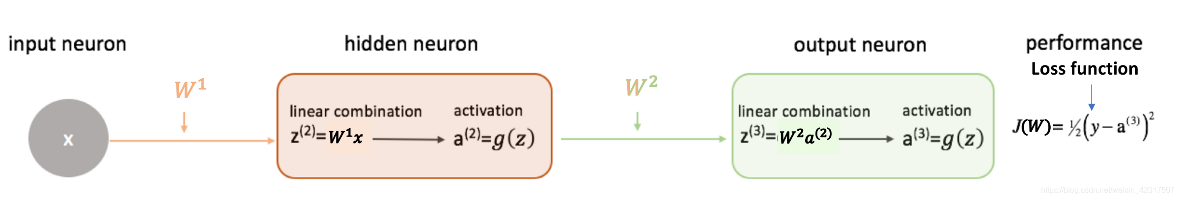
如图, 前馈神经网络(feedforward neural network)是种比较简单的神经网络,只有输入层input layer (黄)、隐藏层hidden layer (绿)、输出层output layer (红)
1.2 激活函数(Activation Function)
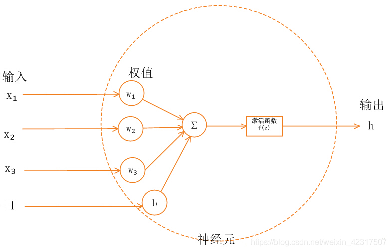
如上图,神经网络神经元中,上层节点的输入值从通过加权求和后,到输出下层节点之前,还被作用了一个函数,这个函数就是激活函数(activation function),作用是提供网络的非线性建模能力。
更直观的图:

每一个神经元如同工厂的流水车间的机器,它重复做着四件事情:【接受上一层数据作为输入>>线性变换>>激活变换>>输出数据到下一层】,每个神经元中有三个组成部分:权重(weight)矩阵W,偏置(bias)向量b,以及激活函数(activation function) g
1.2.1 weights, bias和activation function的作用
why weights and bias?
- Weights shows the strength of the particular node.
- A bias value allows you to shift the activation function curve up or down.
why activation function?
- It is used to determine the output of neural network like yes or no. It maps the resulting values in between 0 to 1 or -1 to 1 etc. (depending upon the function).
1.3 如何形象的解释为什么神经网络层数越多效果越好?
比如某个神经元接收了来自它前一层的身高,体重两个输入,经过加权后,通过带激活阈值(偏置)后的激活函数,输出了一个新的值,这个值的抽象含义可能被解释为“身材匀称度”;
另一个神经元接也收来自它前一层的眼睛大小,嘴巴大小输入,也经过加权、偏置和激活函数,输出了一个新的值,这个值的抽象含义可能被解释为“五官端正度”;
这前一层抽象的“身材匀称度”和“五官端正度”以及其他更多的特征又会继续被输入下一层被以同样的方法处理,得出更多更高层次的抽象特征,比如“帅气度”,随着隐藏层的加深,深层的抽象特征可能抽象得连设计者自己也无法解释。
最后通过层层特征的抽象和输出,神经网络作出它对输入特征的分类——这个人是谁:吴彦祖还是八两金还是其他阿猫阿狗。
可见,浅层神经网络可以表示的特征抽象程度不高,而层次越深,特征的抽象程度越高,也就是在某些特定任务上所谓的“效果越好”,这也是为什么深度神经网络可以做出很多只有人类才能做到的需要高度抽象理解能力的事情。
From:黄卓驹
2. 感知机相关;利用tensorflow等工具定义简单的几层网络(激活函数sigmoid),递归使用链式法则来实现反向传播。
2.1 什么是感知机?
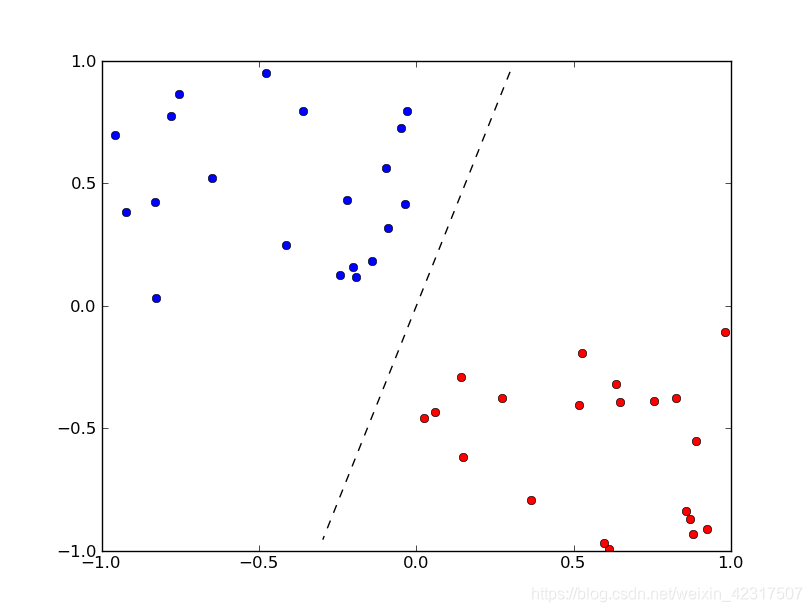
感知机是二分类的线性分类模型,属于监督学习,用于分类。
简单说:
感知机 = 一层的神经网络
好几层的感知机 = 神经网络
假设有一次考试,分为语文,数学,英语,满分都是100分。但是,语文,数学,英语占的权重(weight)不一样。同时,我们还需要根据考试难度,在最后总分上面,进行一些加分或者减分的调整(bias)。最后,根据一个标准(激活函数 Step Function)来定考试合格或者不合格(output)。
如果教务处说,我们是外国语学校,对于英语成绩比较看重,则我们给予这样的英语比较高的权重。
X1:语文成绩 W1:0.3
X2:数学成绩 W2:0.2
X3:英语成绩 W3: 0.5
然后,由于这次考试难度比较高,则每个人都加5分 (这个其实叫做 偏置项 bias)
X0 = 1 W0 = 5
成绩 = X0 * W0 + X1 * W1 + X2 * W2 + X3 * W3
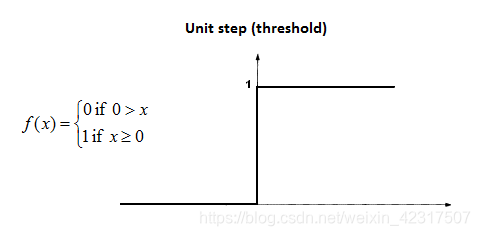
然后,如果成绩为60分及以上则为合格。(激活函数 Step Function)
如果 成绩 >= 60 ,则合格
成绩 < 60 ,则不合格
OK,这样一个简单的感知机就做成了。在权重(W0,W1,W2,W3)和 Step Function(合格标准)定下来的时候,它可以根据输入(各科成绩),求得输出(是否合格)了。
例如:
语文成绩 50 * 0.3 = 15
数学成绩 40 * 0.2 = 8
英语成绩 80 * 0.5 = 40
附加分 5
成绩 15 + 8 + 40 + 5 = 68 =>合格
语文成绩 80 * 0.3 = 24
数学成绩 50 * 0.2 = 10
英语成绩 40 * 0.5 = 20
附加分 5
成绩 24 + 10 + 20 + 5 = 59 => 不合格
当然,一般来讲,感知机往往是激活函数(StepFunction)是事先决定的,作为训练数据的输入,输出是已知的,权重则是需要通过机器学习来获得的。我们的例子中,合格标准是事先决定的,60分及格,然后给出一部分数据:某些人的语文成绩,数学成绩,英语成绩 ,是否合格,然后通过机器学习,将各科的权重计算出来,获得一个模型。然后利用这个模型,通过输入 语文成绩,数学成绩,英语成绩,来判定是否合格。
当然,如果在训练数据比较少的时候,这个权重可能计算的不是很准确,数据越多,权重越准确。
语文成绩 50 数学成绩 40 数学成绩 40 附加分 5 合格
语文成绩 80 数学成绩 50 数学成绩 40 附加分 5 不合格
能够满足这样条件的权重有很多很多,所以机器学习的结果可能不是很好。
但是如果有足够的数据,则权重的计算结果则会非常理想。
最后再回来说一下,为什么叫感知机,其实最简单的,最原始的时候,感知机的输出就是 0(不合格) 或者 1(合格).结果能被感知,或者不能被感知。当然,随着研究的深入,则输出形式也越来越丰富了,不仅限于是否,也可以是数值或者其他形式的东西。例如,感知机做线性回归的时候,则是数值作为输出。
2.2 认识感知机
第一步:输入向量和权重进行点乘,假设叫做k
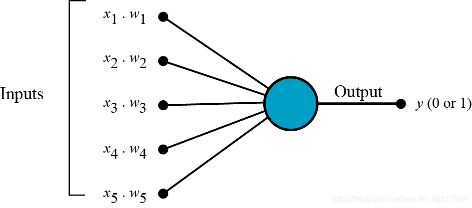
第二步:把所有的k都加起来得到加权和
第三步:将其扔入激活函数中(下图为单位阶跃函)
使用场景:
2.3 建立简单的神经网络
- 利用tensorflow建立简单的三层网络(输入/隐藏/输出)(激活函数sigmoid)参考
import tensorflow as tf
import numpy as np

print('building a neural network...')
#创建一个神经网络
def add_layer(inputs,in_size,out_size,activation_function=None):

    """
    :param input: 数据输入
    :param in_size: 输入大小(即前一层神经元个数)
    :param out_size: 输出大小(即本层神经元个数)
    :param activation_function: 激活函数(默认没有,因为输入层无激活函数)
    """

    Weights = tf.Variable(tf.random_normal([in_size,out_size])) #权值初始化:in_size * out_size
    biases = tf.Variable(tf.zeros([1,out_size])+0.1) #权值初始化初始化:out_size(即本层神经元个数)
    Wx_plus_b = tf.matmul(inputs,Weights)+biases #inputs * Weight + biases
    #按照是否有激活函数,输出:
    if activation_function is None:
        outputs = Wx_plus_b
    else:
        outputs = activation_function(Wx_plus_b)
    return outputs

print( )

print('preparing data...')
x_data = np.linspace(-1,1,300)[:,np.newaxis] #创建输入数据 [-1,1]区间,300个单位,np.newaxis分别是在列(第二维)上增加维度,原先是(300,)变为(300,1)
noise = np.random.normal(0,0.05,x_data.shape) #噪点
y_data = np.square(x_data) - 0.5 + noise #输入对应的输出
y_data=np.square(x_data)+1+noise
print('fertig!')

#define placeholder for inputs to network
#placeholder描述等待输入的节点,只需要指定类型即可
xs = tf.placeholder(tf.float32,[None,1])
ys = tf.placeholder(tf.float32,[None,1])
print('placehoder fertig!')
#三层神经,输入层(1个神经元),隐藏层(10神经元),输出层(1个神经元)
hidden_layer1 = add_layer(xs,1,10,activation_function=tf.nn.sigmoid) #隐藏层
prediction = add_layer(hidden_layer1,10,1,activation_function=None) #输出层
print('hidden layer fertig! output layer fertig!')
#the error between prediciton and real data
#损失函数
loss=tf.reduce_mean(tf.reduce_sum(tf.square(ys-prediction) ,reduction_indices=[1] ))
#选择 optimizer 使 loss 达到最小
train_step=tf.train.GradientDescentOptimizer(0.1).minimize(loss) #学习效率为0.1,梯度下降法使误差最小
print('optimizer fertig!')
#前面是定义,在运行模型前先要初始化所有变量:
init=tf.global_variables_initializer()
#接下来把结构激活,session像一个指针指向要处理的地方:
sess=tf.Session()
#执行初始化
sess.run(init)
print('session initialized')

# 迭代 1000 次学习,sess.run optimizer
for i in range(1000):
   # training train_step 和 loss 都是由 placeholder 定义的运算,所以这里要用 feed 传入参数
   sess.run(train_step, feed_dict={xs: x_data, ys: y_data})
   if i % 50 == 0:
       # to see the step improvement
       print(sess.run(loss, feed_dict={xs: x_data, ys: y_data}))

sess.close()
2.4 反向传播 (Backpropagation)
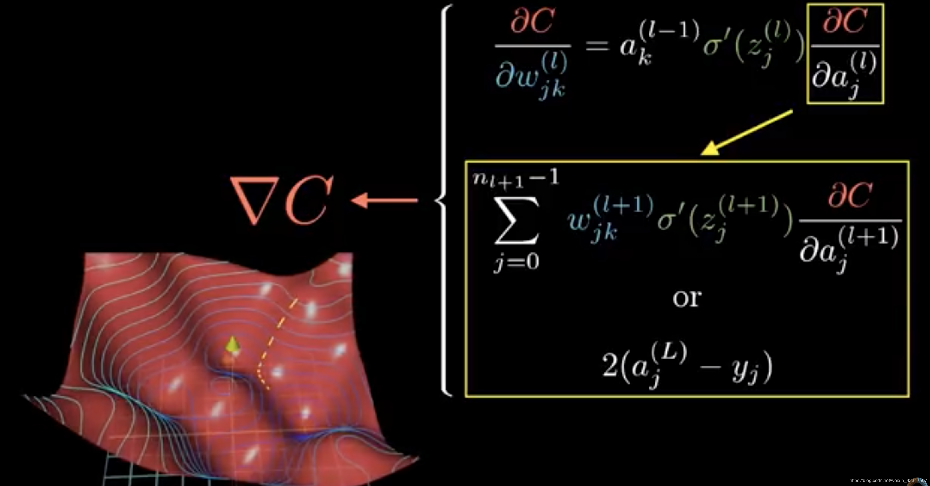
2.4.1 反向传播4大公式
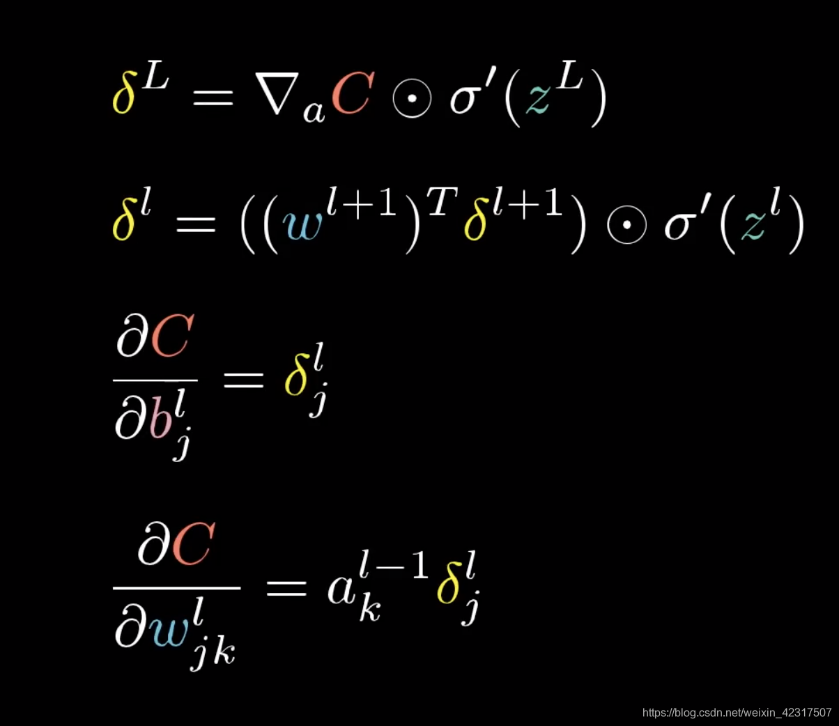
2.4.2 图解反向传播
直观理解反向传播:如下图,是个没被训练好的神经网络(NN),我们用2来举例。在这个NN里,2才0.2,我们希望它升,其他的下降。2
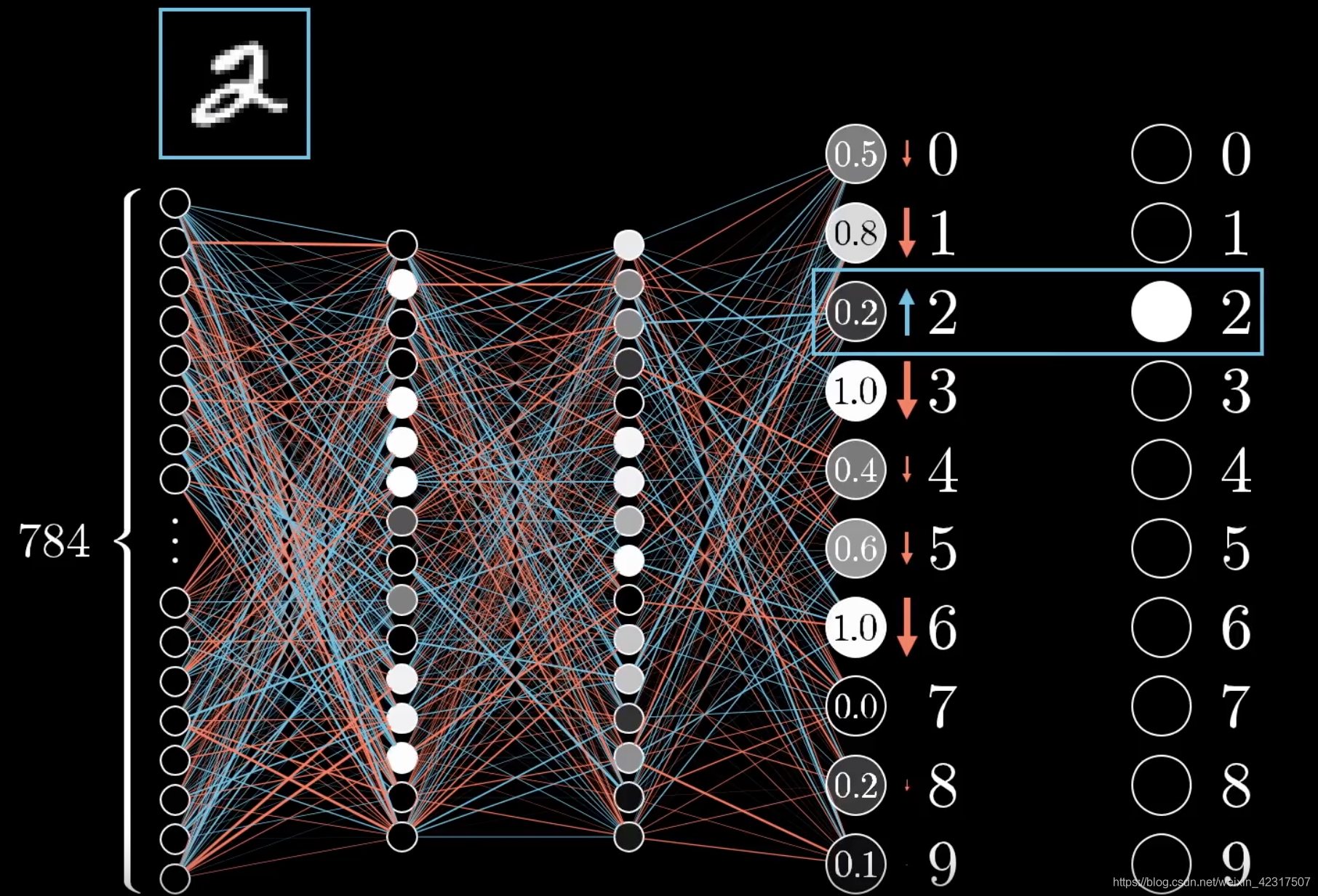
我们把2单独拿出来,想要提升,可以动的有三个值,权重,偏差和上一层的输入。上一层输入的a数值越大,图片里的cell就越亮,所以跟亮cell乘的权重的分量就比跟暗的乘的分量重。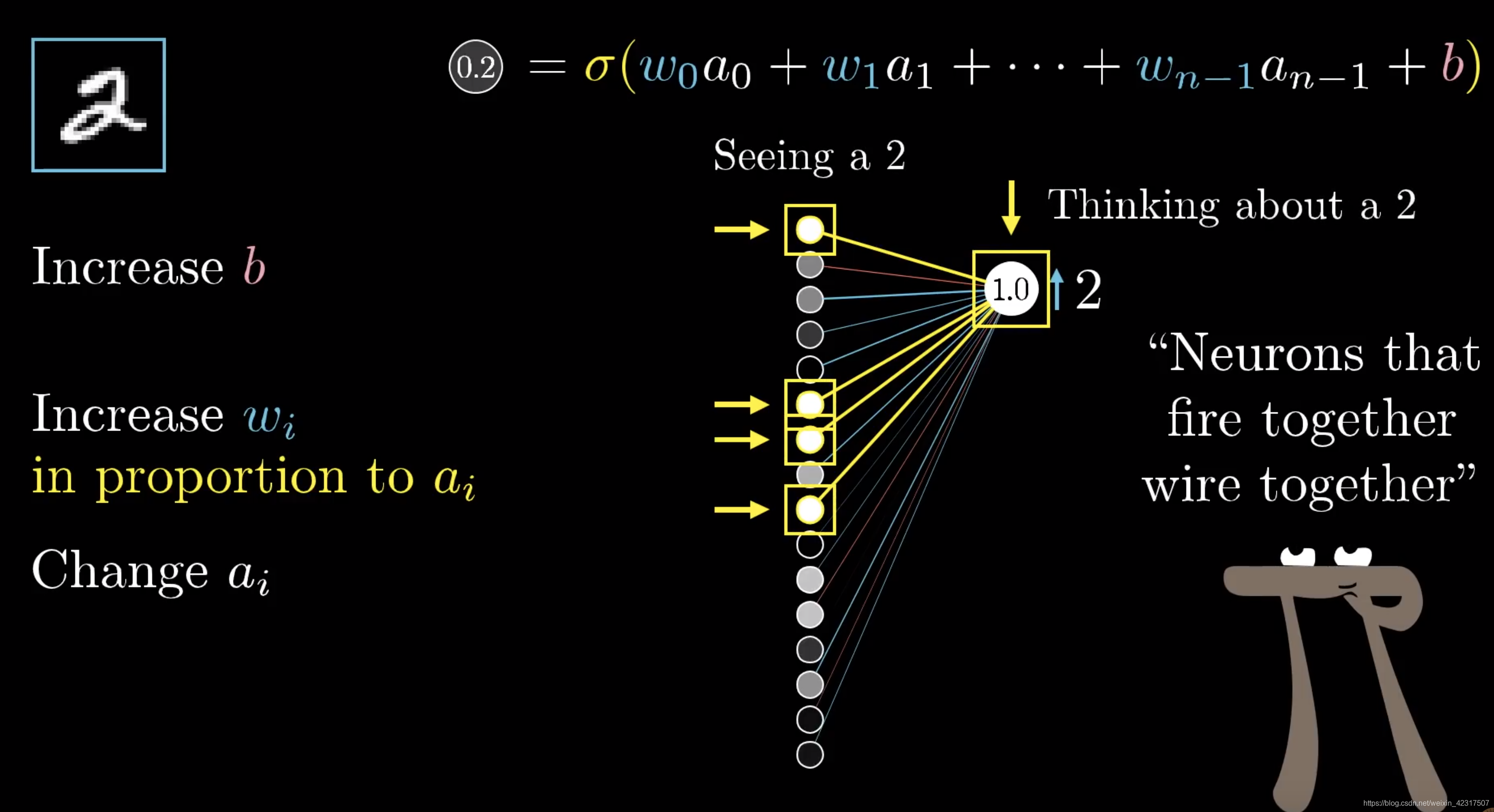
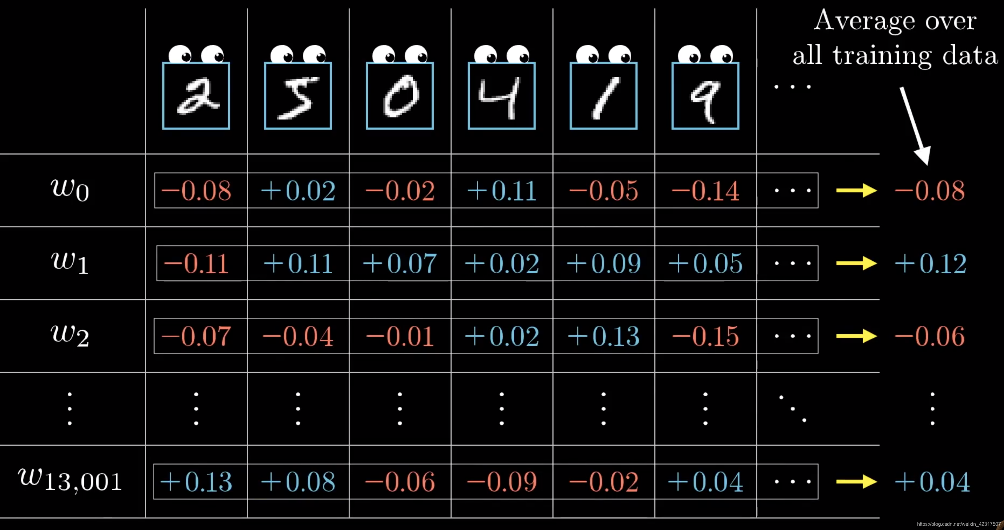
不只是2,其他数字也要调整,这样叠加起来,得到到底要升多少,降多少。
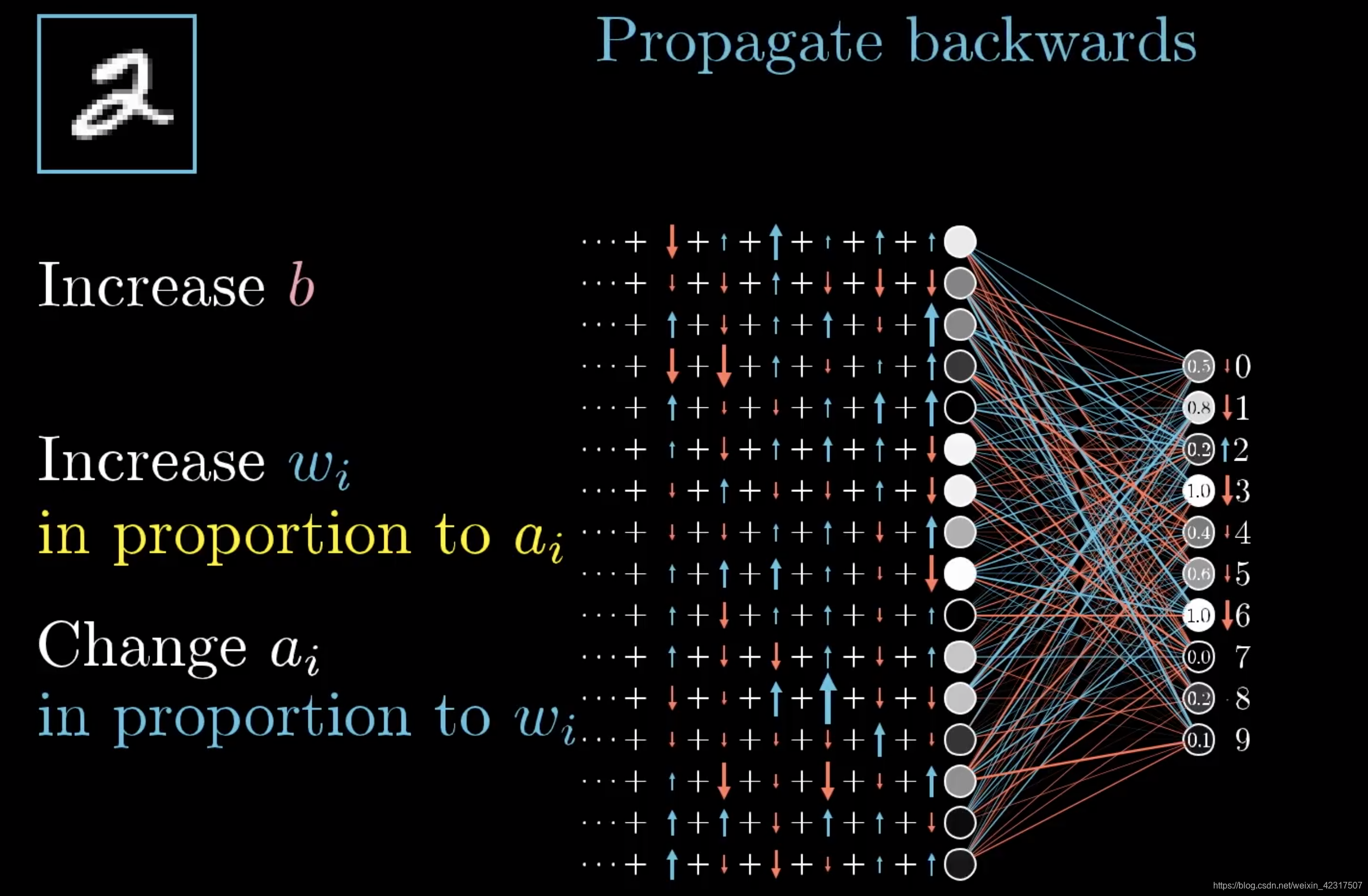
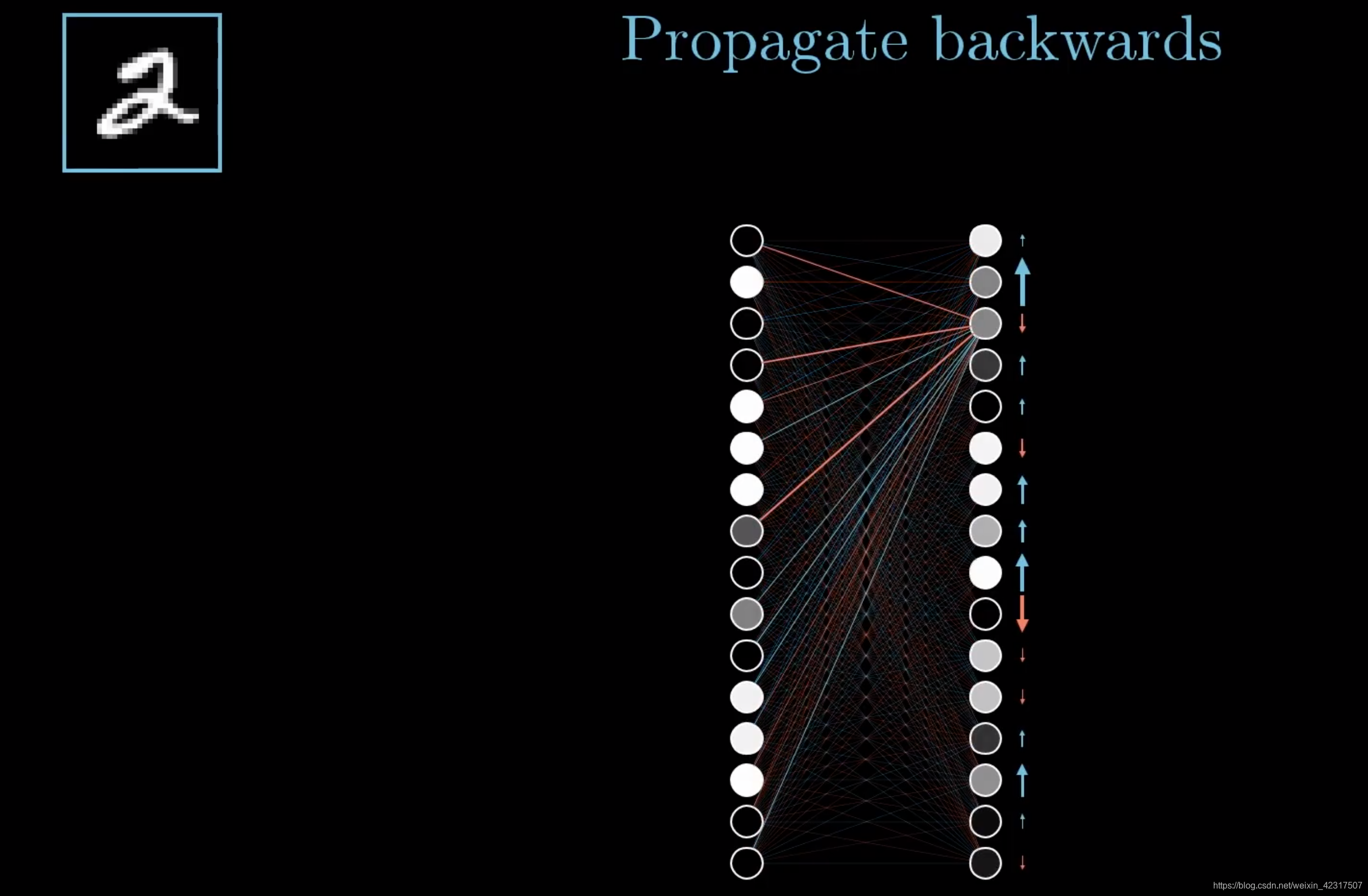
然后对上一层再做一遍刚才做的不可描述之事。
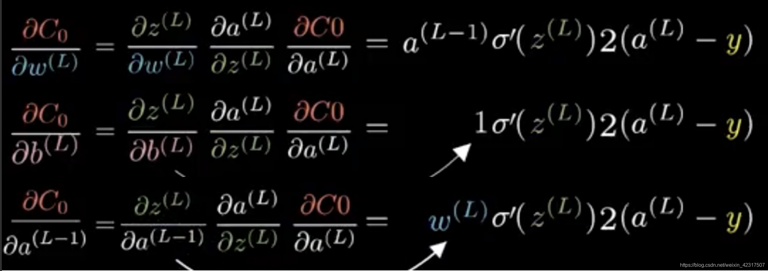
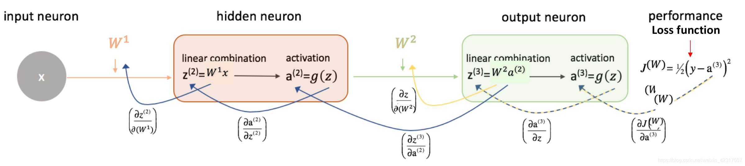
2.4.3 链式法则(Chain Rule)
这就是大概的intuition:先将误差反向传播至隐层,然后再应用梯度下降(gradient descent),其中将误差从末层往前传递的过程需要链式法则(chain rule)的帮助,因此反向传播算法可以说是梯度下降在链式法则中的应用:
一层单个神经元的链式(chain rule):

链式求导:
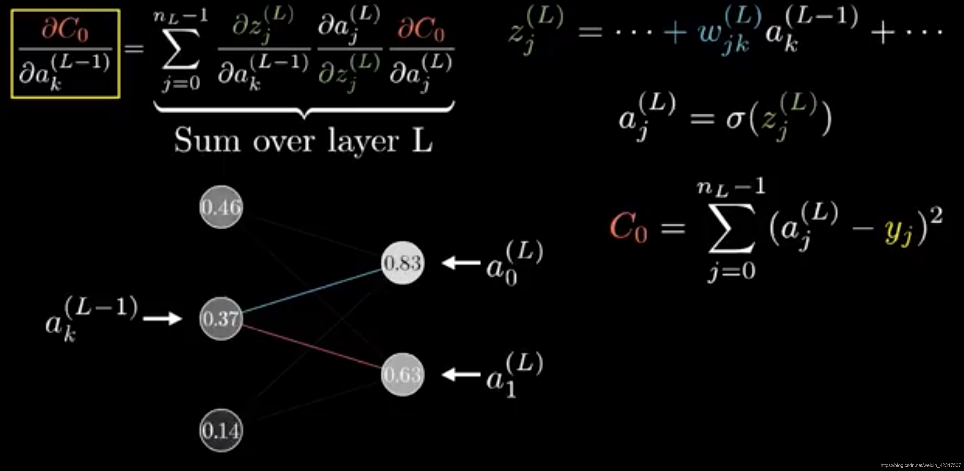
一层多个神经元的链式(chain rule):
3. 激活函数的种类以及各自的提出背景、优缺点。(和线性模型对比,线性模型的局限性,去线性化)
3.1 为什么使用激活函数
Why use?
之所以要在线性变换之后进行非线性变化,是因为,如果没有非线性变换,纯粹使用线性变化的话,不管使用了多少层的线性变换,最终的结果通过合并同类项之后仍然是线性变换,100层的神经网络和1层的没有任何差别。神经网络从本质上来说就是一系列的非线性变换。
3.2 激活函数的挑选
举例:
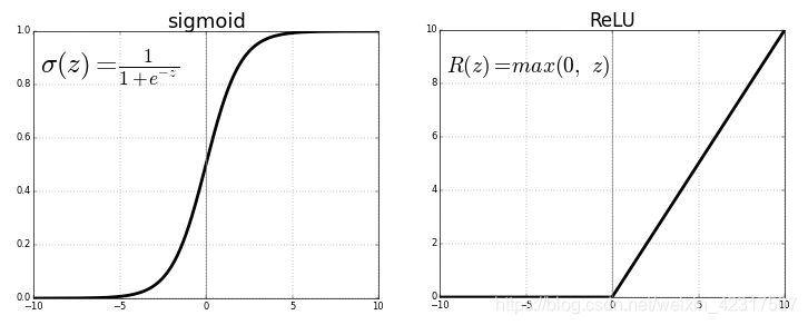
识别预测某张图像是不是一只喵的图像,这里的返回值应该是范围在0~1之间的概率值,sigmoid的函数范围是(0, 1), tanh是(-1, 1), relu是[0, +∞),所以使用sigmoid合适。
从定义来看,几乎所有的连续可导函数都可以用作激活函数(Activation Function)。早期研究神经网络主要采用sigmoid函数或者tanh函数,输出有界,很容易充当下一层的输入。近些年Relu函数及其改进型(如Leaky-ReLU、P-ReLU、R-ReLU等)在多层神经网络中应用比较多:
3.3 激活函数的种类与对比
sigmoid和tanh都用在前馈神经网络:
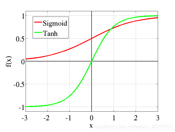
tanh解决了sigmoid不是zero-centered输出问题,但是梯度消失(gradient vanishing)和幂运算的问题仍然存在
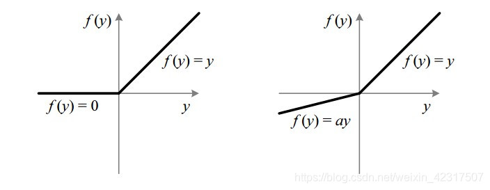
ReLU (Rectified Linear Unit) 现在最常用的激活函数:
问题举例:一个非常大的梯度流过一个 ReLU 神经元,更新过参数之后,这个神经元再也不会对任何数据有激活现象了,那么这个神经元的梯度就永远都会是 0.
如果 learning rate 很大,那么很有可能网络中的 40% 的神经元都”dead”了。
Leaky ReLU是为了解决dying ReLU problem:
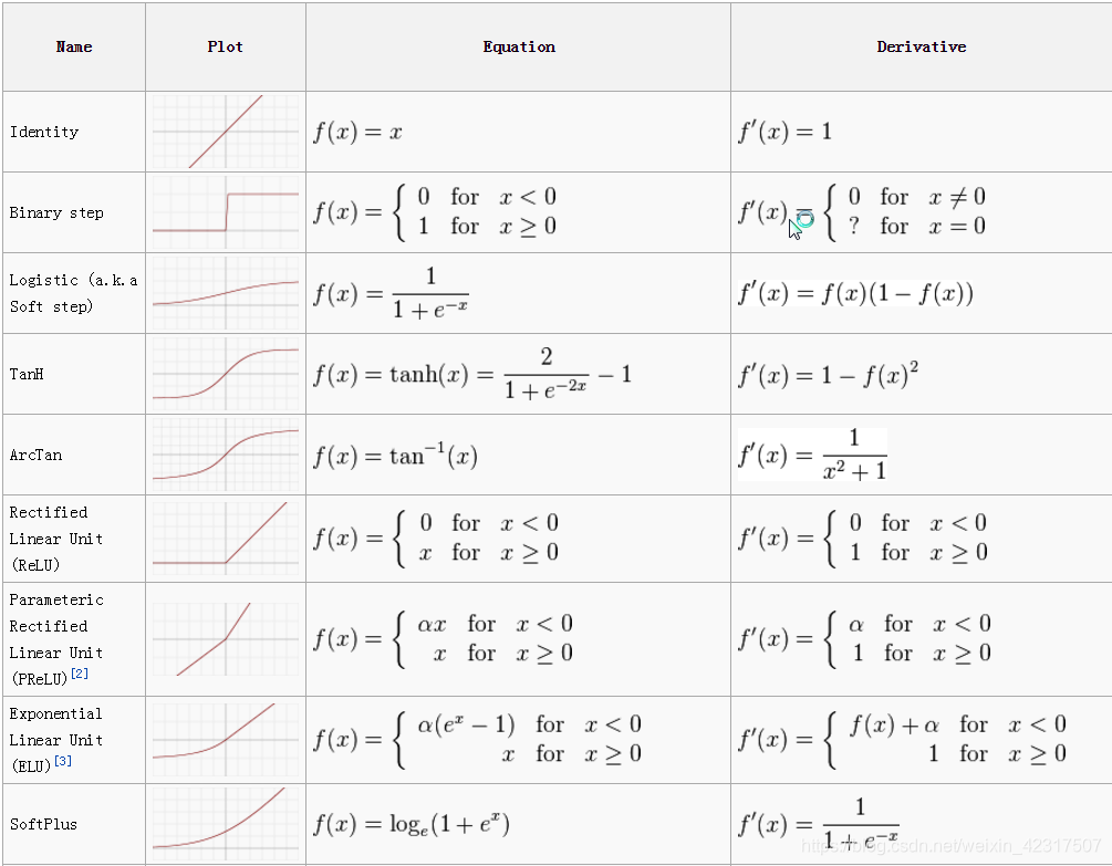
3.4 激活函数的Cheetsheet
直接放个cheetsheet
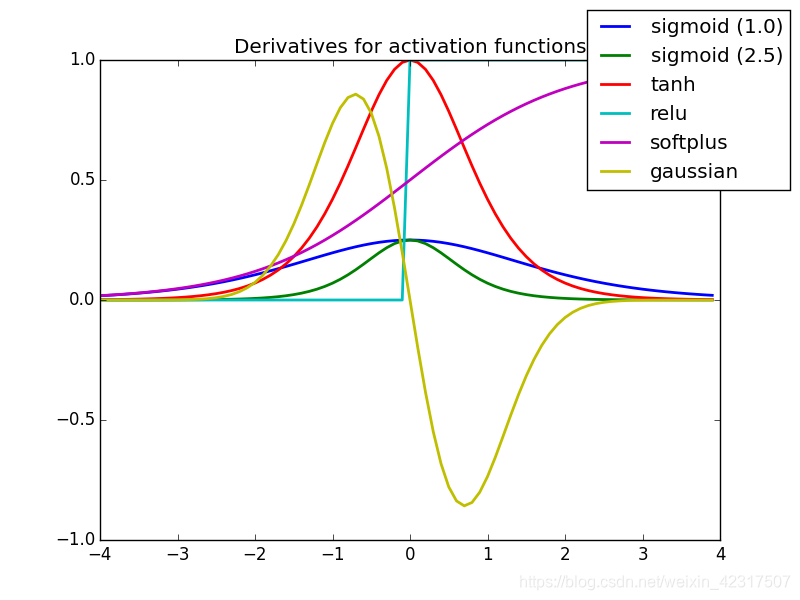
3.5 激活函数的导数图
4. 深度学习中的正则化(参数范数惩罚:L1正则化、L2正则化;数据集增强;噪声添加;early stop;Dropout层)、正则化的介绍。
4.1 什么是正则化?
如下两张图,模型复杂度越往右越复杂,虽然训练误差变小单测试误差变大。
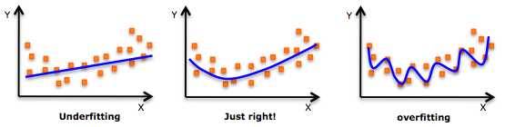
模型在训练集上的训练误差与在测试集上的测试误差的变化趋势对比图:
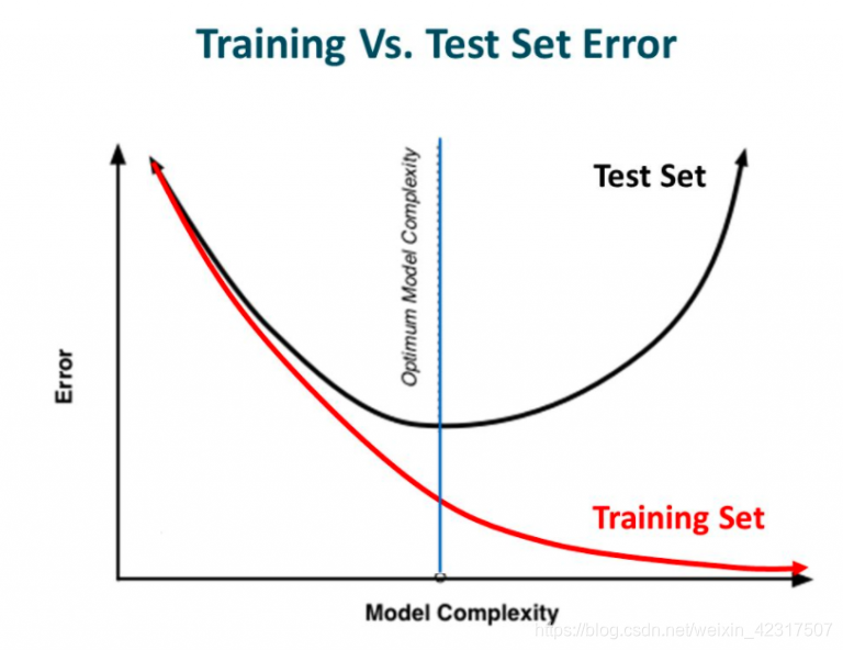
避免过拟合可以使用正则化,在学习过程中降低模型复杂度,提高模型的泛化能力。
there are few ways you can avoid overfitting your model on training data like cross-validation sampling, reducing number of features, pruning, regularization etc.
4.2 正则化原理
机器学习中,正则化就是惩罚系数;在深度学习中,一般是就是惩罚权重:
引入正则项后,会使权重小的特征的权重损失得更多的,而对权重大的特征的权重相对来说损失的就少很多。
不那么合适的举例:
train:英俊潇洒年少多金狂狷邪魅的女人,芳菲妩媚狂狷邪魅的女性友人,风流倜傥玉树临风的美人,
test:皎若秋月出水芙蓉端丽冠绝环肥燕瘦丹唇外朗的女性
没训练好的模型是狂狷邪魅权重大,上帝视角看,权重大的特征是应该是女的,正则就是把狂狷邪魅的系数多缩一缩,别碍事。
4.3 正则化的种类
4.3.1 L2 and L1 regularization
- L1 Regularization (Lasso Regression Lasso回归)
- L2 Regularization (Ridge Regression 岭回归)
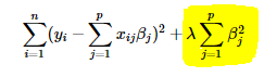
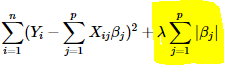
- L2 Regularization
岭回归是给原来的损失函数加上
的平方作为惩罚项:
 图源
图源
是调整因子,它决定了我们要如何对模型的复杂度进行惩罚。如果
为零,就回到了OLS(普通最小二乘);如果
倍儿大,会导致欠拟合。所以
的值如何选很重要。岭回归用在避免过拟合上棒棒的。
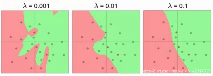
如图,λ=0.001, 惩罚程度不够,过拟合
- L1 Regularization
Lasso(Least Absolute Shrinkage and Selection Operator) 是给原来的损失函数加上
的绝对值作为惩罚项:
同样的,如果
为零,就回到了OLS;如果值太大,会导致欠拟合。
- L1与L2的区别
Lasso把不那么重要的特征的系数收缩为零。让这些特征说再见。所以,有巨多特征时,特征选择请找Lasso(产生稀疏模型)。
4.3.2 Dropout
防止过拟合还有个方法叫dropout。
The term “dropout” refers to dropping out units (hidden and visible) in a neural network. By dropping a unit out, we mean temporarily removing it from the network, along with all its incoming and outgoing connections.1
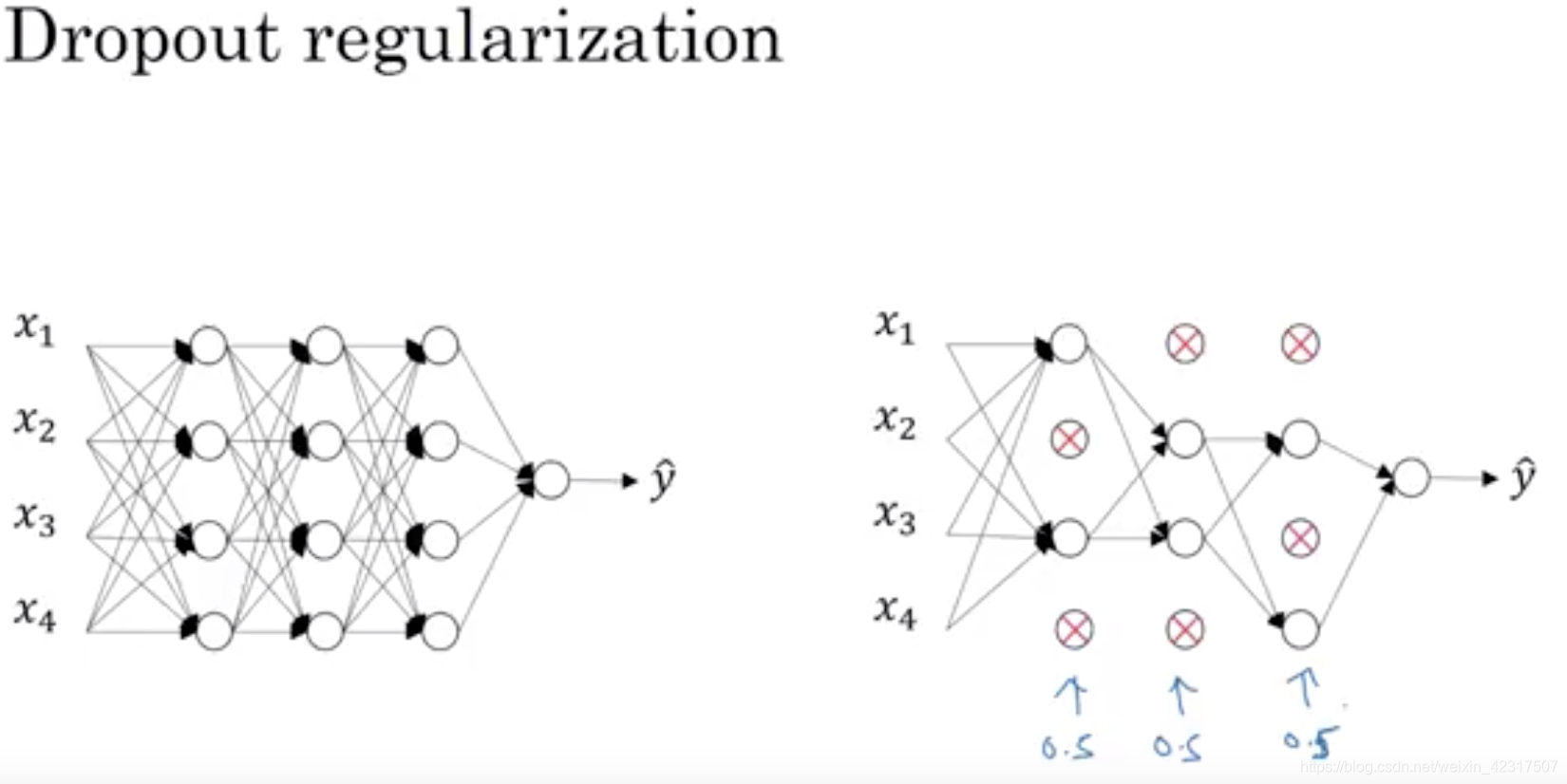
一般用于特别大的神经网络,以某种概率随机选择神经元扔掉,当然每次迭代时,扔的神经元都不一样,这样就不会太依赖某些邪魅狂狷的特征,提升模型的泛化能力。图中的0.5就是dropout的概率,四个里扔俩。
缺点:A dropout network typically takes 2-3 times longer to train than a standard neural network of the same ar- chitecture. 1
4.3.3 Data augmentation
防止过拟合还可以扩大数据集,常用于图片识别。
举例:

如上图,左边是品牌A,右边是品牌B。训练集里各种颜色的品牌A都是朝向左,品牌B都是朝向右。心大的进行训练,测试时候扔进去一张朝向左的品牌A,自己觉得模型非常完美。然后扔入一张朝向右的品牌A,如下图:

这时候模型给出结果是品牌B,瞬间凉凉。
怎么办?我们就可以运用augmentation,让训练集的图片变化各种姿势:flip, rotation, crop, scale, translation, Gaussian Noise, etc. 3

当然,这只是最基本的姿势。
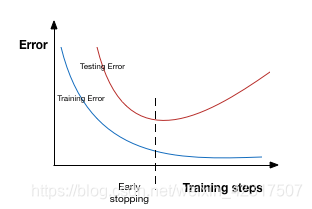
4.3.4 Early stopping
过拟合之前喊停,结束训练。
Early stopping is a kind of cross-validation strategy where we keep one part of the training set as the validation set. When we see that the performance on the validation set is getting worse, we immediately stop the training on the model.
如图:
5. 深度模型中的优化:参数初始化策略;自适应学习率算法(梯度下降、AdaGrad、RMSProp、Adam;优化算法的选择);batch norm层(提出背景、解决什么问题、层在训练和测试阶段的计算公式);layer norm层。
5.1 参数初始化
再回顾一遍基本操作:
Consider an L layer neural network, which has L-1 hidden layers and 1 output layer.
- weight matrix of dimension (size of layer l, size of layer l-1)
- bias vectors of dimension (size of layer l, 1)
- Linear activations at layer 1
- Non-linear function
- Non-linear activations: output of
, where
is the input data
训练神经网络分四步:
- Initialize weights and biases.
- Forward propagation: Using the input X, weights W and biases b, for every layer we compute Z and A. At the final layer, we compute f(A^(L-1)) which could be a sigmoid, softmax or linear function of A^(L-1) and this gives the prediction y_hat.
- Compute the loss function: This is a function of the actual label y and predicted label y_hat. It captures how far off our predictions are from the actual target. Our objective is to minimize this loss function.
- Backward Propagation: In this step, we calculate the gradients of the loss function f(y, y_hat) with respect to A, W, and b called dA, dW and db. Using these gradients we update the values of the parameters from the last layer to the first.
- Repeat steps 2–4 for n iterations/epochs till we feel we have minimized the loss function, without overfitting the train data (more on this later!)
Here’s a quick look at steps 2 , 3 and 4 for a network with 2 layers, i.e. one hidden layer. (Note that I haven’t added the bias terms here for simplicity):
5.1.1 Weight Initialization
- 初始化权重矩阵为0
相当于线性模型了。
It is important to note that setting biases to 0 will not create any troubles as non zero weights take care of breaking the symmetry and even if bias is 0, the values in every neuron are still different.
- 初始化权重矩阵随机
np.random.randn(size_l, size_l-1)会产生两个问题:
a) Vanishing gradients 梯度消失
b) Exploding gradients 梯度爆炸
- 实战:
1. 用 RELU/ leaky RELU 作为激活函数
像leaky RELU没有0梯度,神经元不会死掉。
2. 启发式
use heuristic to initialize the weights depending on the non-linear activation function
a) For RELU(z)
— We multiply the randomly generated values of W by:
= np.random.randn(size_1, size_l-1) *np.sqrt(2/size_l-1)
b) For tanh(z) (Xavier initialization)
— The heuristic is called Xavier initialization. It is similar to the previous one, except that k is 1 instead of 2.
= np.random.randn(size_1, size_l-1) *np.sqrt(1/size_l-1)
#In TensorFlow :
initializer = tf.contrib.layers.xavier_initializer()
W = tf.get_variable('W', [dims], initializer)
c) Another commonly used heuristic is:
= np.random.randn(size_1, size_l-1) *np.sqrt(2/(size_l-1+size_l))
3. Gradient Clipping 梯度裁剪
用于应对梯度爆炸。
We set a threshold value, and if a chosen function of a gradient is larger than this threshold, we set it to another value. For example, normalize the gradients when the L2 norm exceeds a certain threshold –
W = W * threshold / l2_norm(W) if l2_norm(W) > threshold
5.2 优化算法
都在这里:An overview of gradient descent optimization algorithms -Sebastian Ruder
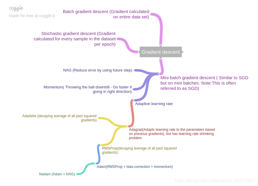
In summary, SGD suffers from 2 problems: (i) being hesitant at steep slopes, and (ii) having same learning rate for all parameters. So the improved algorithms are categorized as:
- Momentum, NAG: address issue (i). Usually NAG > Momentum.
- Adagrad, RMSProp: address issue (ii). RMSProp > Adagrad.
- Adam, Nadam: address both issues, by combining above methods.
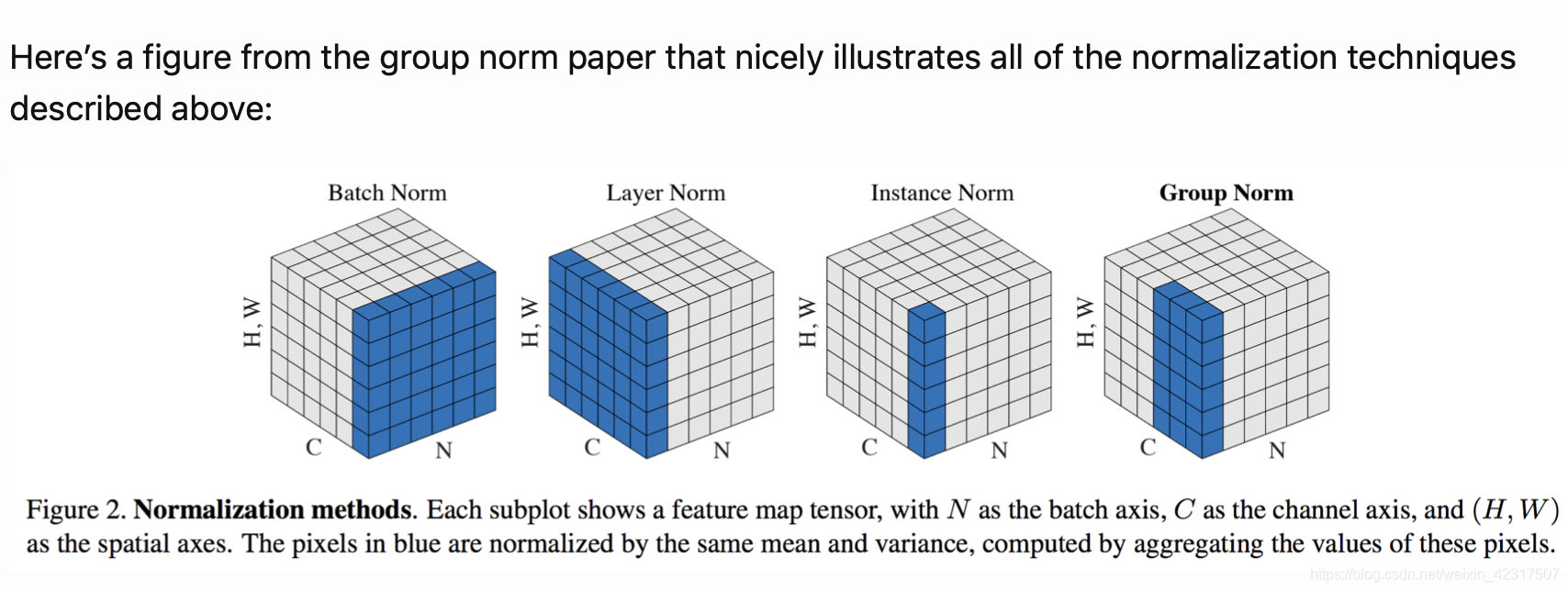
5.3 归一化
Batch Normalization(2015年)
Layer Normalization(2016年)
5.3.1 Batch normalization
看这里:Batch Normalization: Accelerating Deep Network Training by Reducing Internal Covariate Shift
The goal of batch norm is to reduce internal covariate shift by normalizing each mini-batch of data using the mini-batch mean and variance.
import tensorflow as tf

is_train = tf.placeholder(tf.bool, name="is_train");

x_norm = tf.layers.batch_normalization(x, training=is_train)

update_ops = tf.get_collection(tf.GraphKeys.UPDATE_OPS)
with tf.control_dependencies(update_ops):
    train_op = optimizer.minimize(loss)
5.3.2 Layer normalization
看这里:Layer Normalization
Layer norm attempted to address some shortcomings of batch norm:
- It’s unclear how to apply batch norm in RNNs
- Batch norm needs large mini-batches to estimate statistics accurately
总结如图: