这是一个简单的快速开始在喀拉什神经网络中执行数字识别，为一个简短的教程。

import numpy as np
import matplotlib.pyplot as plt
plt.rcParams['figure.figsize'] = (7,7) # Make the figures a bit bigger

from keras.datasets import mnist
from keras.models import Sequential
from keras.layers.core import Dense, Dropout, Activation
from keras.utils import np_utils
%matplotlib inline

F:\anaconda\lib\site-packages\h5py\__init__.py:34: FutureWarning: Conversion of the second argument of issubdtype from `float` to `np.floating` is deprecated. In future, it will be treated as `np.float64 == np.dtype(float).type`.
  from ._conv import register_converters as _register_converters
Using TensorFlow backend.

加载训练数据

nb_classes = 10

# the data, shuffled and split between tran and test sets
(X_train, y_train), (X_test, y_test) = mnist.load_data()
print("X_train original shape", X_train.shape)
print("y_train original shape", y_train.shape)

X_train original shape (60000, 28, 28)
y_train original shape (60000,)

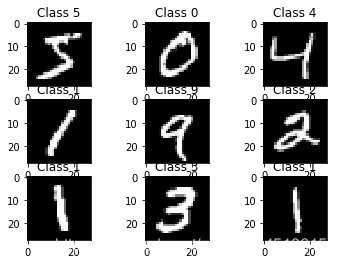
看看训练数据的一些示例

for i in range(9):
    plt.subplot(3,3,i+1)
    plt.imshow(X_train[i], cmap='gray', interpolation='none')
    plt.title("Class {}".format(y_train[i]))

在这里插入图片描述

设置数据格式

我们的神经网络将为每个训练示例采用一个向量，因此我们需要重新调整输入，使每个28x28图像成为单个784维向量。我们还将缩放输入到范围[0-1]而不是[0-255]

X_train = X_train.reshape(60000, 784)
X_test = X_test.reshape(10000, 784)
X_train = X_train.astype('float32')
X_test = X_test.astype('float32')
X_train /= 255
X_test /= 255
print("Training matrix shape", X_train.shape)
print("Testing matrix shape", X_test.shape)

Training matrix shape (60000, 784)
Testing matrix shape (10000, 784)

将目标矩阵修改为一个热格式，即

0 -> [1, 0, 0, 0, 0, 0, 0, 0, 0]
1 -> [0, 1, 0, 0, 0, 0, 0, 0, 0]
2 -> [0, 0, 1, 0, 0, 0, 0, 0, 0]
etc.

Y_train = np_utils.to_categorical(y_train, nb_classes)
Y_test = np_utils.to_categorical(y_test, nb_classes)

#建立神经网络

建立神经网络。这里我们将做一个简单的3层完全连接的网络。
在这里插入图片描述

model = Sequential()
model.add(Dense(512, input_shape=(784,)))
# “激活”只是应用于输出的非线性函数。
#上一层的。这里，有一个“整流线性单元”，
#我们将所有值都限制在0到0之间。
model.add(Activation('relu')) 
                           
model.add(Dropout(0.2))   # Dropout 有助于保护模型不被记忆或“过拟合”训练数据。
model.add(Dense(512))
model.add(Activation('relu'))
model.add(Dropout(0.2))
model.add(Dense(10))
#这个特殊的“softmax”激活等等，
#确保输出是有效的概率分布，即
#它的值都是非负的，和为1。
model.add(Activation('softmax'))

编译模型

Keras构建在Ano（现在也是TensorFlow）之上，这两个包都允许您在python中定义一个计算图，然后它们在CPU或GPU上高效编译和运行，而不需要python解释器的开销。

在编译模型时，keras要求您指定丢失函数和优化器。我们在这里使用的损失函数称为“分类交叉熵”，它是一个非常适合比较两个概率分布的损失函数。

在这里，我们的预测是10个不同数字的概率分布（例如，“我们80%确信这幅图像是3，10%确定它是8，5%确定它是2，等等”），目标是100%的概率分布，正确的类别，以及0%的概率分布。交叉熵是一个衡量你的预测分布与目标分布有多大不同的指标。[维基百科上的更多细节]（https://en.wikipedia.org/wiki/cross_entropy）

优化器有助于确定模型学习的速度，以及它对“卡住”或“爆炸”的抵抗力。我们不会太详细地讨论这个问题，但是“亚当”通常是一个很好的选择（在U of T开发）。

model.compile(loss='categorical_crossentropy', optimizer='adam')

训练模型！

这是有趣的部分：你可以将之前加载的训练数据输入到这个模型中，它将学习对数字进行分类。

model.fit(X_train, Y_train,
          batch_size=128, nb_epoch=4,
          show_accuracy=True, verbose=1,
          validation_data=(X_test, Y_test))

Train on 60000 samples, validate on 10000 samples
Epoch 1/4
60000/60000 [==============================] - 10s - loss: 0.2521 - acc: 0.9245 - val_loss: 0.1131 - val_acc: 0.9651
Epoch 2/4
60000/60000 [==============================] - 10s - loss: 0.1016 - acc: 0.9687 - val_loss: 0.0827 - val_acc: 0.9746
Epoch 3/4
60000/60000 [==============================] - 11s - loss: 0.0711 - acc: 0.9779 - val_loss: 0.0668 - val_acc: 0.9791
Epoch 4/4
60000/60000 [==============================] - 11s - loss: 0.0557 - acc: 0.9816 - val_loss: 0.0642 - val_acc: 0.9805





<keras.callbacks.History at 0x12655bbe0>

最后，评估其性能

score = model.evaluate(X_test, Y_test,
                       show_accuracy=True, verbose=0)
print('Test score:', score[0])
print('Test accuracy:', score[1])

Test score: 0.0642029843267
Test accuracy: 0.9805

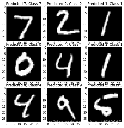
检查输出

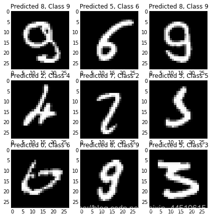
检查输出并确保一切正常是个好主意。在这里，我们将看到一些正确的例子，以及一些错误的例子。

#预测类函数输出最高概率的类

#根据每个输入示例的训练分类器。
predicted_classes = model.predict_classes(X_test)

 

#检查哪些项目是对的/错的
correct_indices = np.nonzero(predicted_classes == y_test)[0]
incorrect_indices = np.nonzero(predicted_classes != y_test)[0]

10000/10000 [==============================] - 0s

plt.figure()
for i, correct in enumerate(correct_indices[:9]):
    plt.subplot(3,3,i+1)
    plt.imshow(X_test[correct].reshape(28,28), cmap='gray', interpolation='none')
    plt.title("Predicted {}, Class {}".format(predicted_classes[correct], y_test[correct]))
    
plt.figure()
for i, incorrect in enumerate(incorrect_indices[:9]):
    plt.subplot(3,3,i+1)
    plt.imshow(X_test[incorrect].reshape(28,28), cmap='gray', interpolation='none')
    plt.title("Predicted {}, Class {}".format(predicted_classes[incorrect], y_test[incorrect]))