【TensorFlow】笔记４：图像识别与CNN

版权声明：本文为博主原创文章，未经博主允许不得转载。 https://blog.csdn.net/u012736685/article/details/88572456

一、图像识别＆经典数据集

图像识别：希望借助计算机程序来处理、分析和理解图片中的内容，使得计算机可以从图片中自动识别各种不同模式的目标和对象。

1、Cifar数据集

Cifar-10：10种不同种类的60000张图像，像素大小为32*32的彩色图像

Cifar-100：20 个大类，大类又细分为 100 个小类别，每类包含 600 张图像。

• Cifar相比MNIST的最大区别：彩色，且每张图包含一个种类的实体分类难度更高。
• 无论Cifar还是MNIST，相比真实环境的图像识别，还有两个主要的问题：
  • 现实生活的图片分辨率远远高于32*32，且分辨率不固定；
  • 现实生活中物体类别很多，且每张图像中不会仅仅出现一种物体；

2、 ImageNet

• 由斯坦福教授李飞飞（Feifei Li）带头整理的数据库，更加贴近真实生活环境。
• Imagenet数据集有1400多万幅图片，涵盖2万多个类别；其中有超过百万的图片有明确的类别标注和图像中物体位置（bounding box）的标注，一张图片中可能出现多个同义词集所代表的实体。
• ILSVRC2012数据集：1000 个类别的 120 万张图片，其中
  每张图片属于且只属于一个类别。

top-N 正确率：图像识别算法给出前 N 个答案中有一个是正确的概率。其中 N 的取值一般为 3 或 5

二、CNN

两者之间最主要的区别就在于相邻两层之间的连接方式

Q1：为什么全连接不能很好的处理图像数据?

最大的问题在于全连接层参数太多，使得计算速度减慢，且容易导致过拟合问题。

Q2：卷积神经网络的优势

在卷积神经网络的前几层中，每一层的节点都被组织成一个三维矩阵，可以看出前几层的每个节点都是和上层中的部分节点相连。

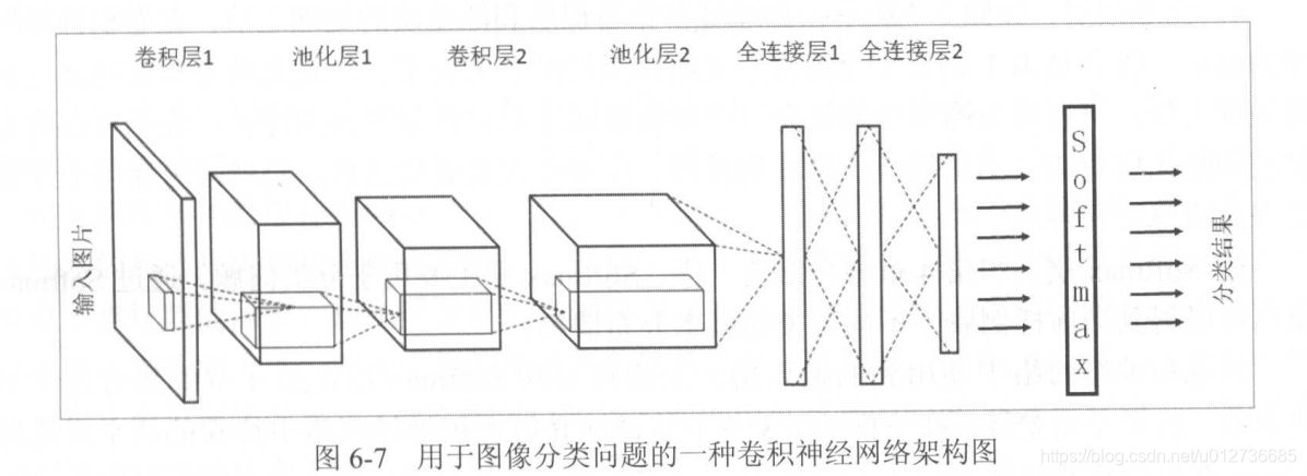
Q3：卷积神经网络由以下五部分构成：

1. 输入层
   输入层是整个神经网络的输入，在图像处理中，输入一般代表一张图片的像素矩阵（常用三维矩阵表示）。三维矩阵的长和宽代表图像的大小，深度代表了图像的色彩通道。从输入层开始，卷积神经网络通过不同的神经网络结构将上一层的三维矩阵转化为下一层的三维矩阵，直到最后的全连接层。

2. 卷积层
   卷积层是卷积神经网络中最重要的部分。卷积层中每一个节点的输入只是上一层神经网络的一小块，这个小块常用的大小有3∗3或5∗5，卷积层试图将神经网络中的每个小块进行更加深入的分析从而抽象得到更高层次的特征，一般来说经过卷积层处理过的节点矩阵会变得更深。

3. 池化层
   池化层神经网络不会改变三维矩阵的深度，但是它可以缩小矩阵的大小。池化层可以进一步缩小最后全连接层中节点的个数，从而达到减少整个神经网络中参数的目的。

4. 全连接层
   经过多轮卷积层和池化层的处理之后，卷积神经网络的最后一般会是由1-2个全连接层来给出最后的分类结果。经过几轮卷积层和池化层处理之后，可以认为图像中的信息已经被抽象成了信息含量更高的特征。 可以将卷积和池化层看成特征提取的过程，提取完成之后，仍然需要使用全连接层来完成分类任务。

5. Softmax层（pooling层）
   Softmax层主要用于分类问题，通过softmax可以得到当前样例属于不同种类的概率分布情况。

三、卷积神经网络常用结构

1、卷积层

TensorFlow文档中将下图的部分被称为“过滤器”或“内核”，过滤器可以将当前层神经网络上的一个子节点矩阵转化为下一层神经网络上的一个单位节点矩阵（长和宽都为1，但深度不限的节点矩阵）。

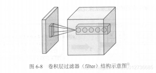
过滤器：

• 常用的过滤器的大小为 33 或 55 的，过滤器处理的矩阵深度和当前层神经网络节点矩阵的深度一致。
• 尺寸：过滤器输入节点矩阵的大小
• 深度：输出节点矩阵的深度
• 上图中，左侧小矩阵的尺寸为过滤器的尺寸，右侧单位矩阵的深度为过滤器的深度。
• 前向传播过程：通过左侧小矩阵的节点计算出右侧单位矩阵中节点的过程

过滤器的前向传播
通过将一个过滤器从神经网络当前层的左上角移动到右下角，并且在移动过程中计算每一个对应的单位矩阵得到的。

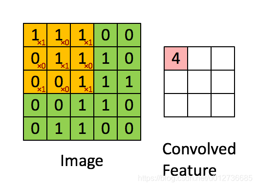
全零填充（zero-padding）：为了避免尺寸变化，可以使用“全零填充”，可以使得前向传播后两矩阵大小不变。

设置不同的步长：也可以调整卷积后矩阵的大小

参数共享：每一个卷积层中使用的滤波器中的参数都是一样的（很重要的性质）

• 使得图像上的内容不受位置的影响，因为一幅图上的滤波器是相同的，无论“1”出现在图中的哪个位置，滤波的结果都是一样的。
• 很大程度上减少神经网络的参数
• 卷积层的参数个数和图片的大小无关，它只和过滤器的尺寸、深度以及当前层节点矩阵的深度有关。
  • 参数个数：过滤器的长×过滤器的宽×当前层节点矩阵的深度×过滤器的深度（输出节点矩阵的深度）+偏置数(=过滤器的深度过滤器的深度)

一个卷积层的前向传播过程

import tensorflow as tf

# 参数变量是一个四维矩阵，
# 分为是过滤器的尺寸（长、宽）、当前层的深度、过滤器的深度
filter_weight = tf.get_variable('weights', [5, 5, 3, 16], initializer=tf.truncated_normal_initializer(stddev=0.1))
# 偏置项也是共享的,参数值为下一层深度个（过滤器的深度）个不同的偏置项
biases = tf.get_variable('biases', [16], initializer=tf.constant_initializer(0.1))

# tf.nn.conv2d实现卷积层前向传播
#  第一个输入：当前层节点矩阵,第一维对应一个输入batch
# （比如输入层，input[0,:,:,:]表示输入第一张图像，input[1,:,:,:]表示输入第二张图像
#  第二个参数：卷积层的权重
#  第三个参数不同维度上的步长（第一维和最后一维要求一定是1，因为步长只对矩阵的长和宽有效）
#  第四个参数：填充的方法，可选'SAME'（全0填充）/'VALID'（不填充）
conv = tf.nn.conv2d(input, filter_weight, strides=[1,1,1,1], padding='SAME')

# tf.nn.bias_add 可以在每一个节点加上偏置项
# 不直接使用加法：因为矩阵上不同位置上的节点都需要加上相同的偏置项
bias = tf.nn.bias_add(conv, biases)
# 将计算结果通过ReLU函数激活
actived_relu = tf.nn.relu(bias)

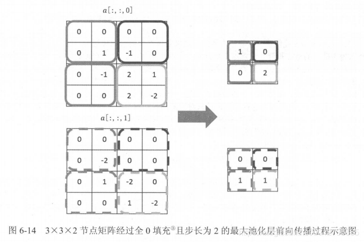
2、池化层

作用：

• 减少参数
• 防止过拟合
• 获得平移不变性
• 加快计算速度

常用池化的类型：

• 最大池化
• 平均池化

池化层的作用范围：

• 只影响一个深度上的节点
• 在长、宽、深这三个维度都要进行移动

（２）实现

实现最大池化层的前向传播

pool = tf.nn.max_pool(actived_conv,ksize[1,3,3,1],strides=[1,2,2,1],padding='SAME')

 # 第一个参数：当前层节点矩阵
 # 第二个参数：过滤器尺寸
 #             给出的是一个长度为4的一位数组，但数组的首位和末位必须为1
 #             意味着池化层的过滤器是不可以跨过不同样例或节点矩阵深度的
 # 第三个参数：步长，第一维和最后一维必须为1，即池化层不能减少节点矩阵的深度或者输入样例的个数
 # 第四个参数：填充方法，'SAME'表示全0填充，'VALID'表示不填充

实现平均池化层的前向传播

pool = tf.nn.avg_pool(actived_conv,ksize[1,3,3,1],strides=[1,2,2,1],padding='SAME')

 # 第一个参数：当前层节点矩阵
 # 第二个参数：过滤器尺寸
 #             给出的是一个长度为4的一维数组，但数组的首位和末位必须为1
 #             意味着池化层的过滤器是不可以跨过不同样例或节点矩阵深度的
 # 第三个参数：步长，第一维和最后一维必须为1，即池化层不能减少节点矩阵的深度或者输入样例的个数
 # 第四个参数：填充方法，'SAME'表示全0填充，'VALID'表示不填充

四、经典CNN模型

通过这些经典的卷积神经网络的网络结构可以总结出卷积神经网络结构设计的一些模式。

1、LeNet-5 模型（1998）

（１）模型

Yann LeCun 教授于1998年提出，是第一个成功用于数字识别的卷积神经网络，在mnist数据集上，可以达到99.2%的效果，共有7层

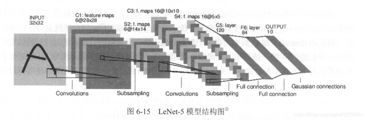
输入原始图像的大小是32×32。

第一层：卷积层

• 输入：原始图像的像素（32×32×1）
• 过滤器：尺寸为 $5\times5$，深度为6，不使用全0填充，步长为1
• 输出：尺寸为 $32-5+1=28$，深度为6
• 参数个数： $5\times5\times1\times6+6=156$
• 下一层节点矩阵的节点： $28\times28\times6=4704$ ，每个节点和 $5\times5=25$ 个当前层节点相连
• 本层卷积层共有连接个数： $28\times28\times6\times(25+1)=122304$

第二层：池化层

• 输入：第一层的输出，是一个 $28\times28\times6$ 的节点矩阵
• 过滤器：大小为2*2，长、宽、步长都为2
• 输出： $14\times14\times6$

第三层：卷积层

• 输入： $14\times14\times6$
• 过滤器：大小为 $5\times5$，深度为16，不使用0填充，步长为1
• 输出： $10\times10\times16$，按标准的卷积层，本层应该有 $5\times5\times16\times+16=2416$个参数
• 共有： $10\times10\times16\times(25+1)=41600$ 个连接

第四层：池化层
输入： $10\times10\times16$
过滤器：大小为 $2\times2$，步长为2
输出：矩阵大小为 $5\times5\times16$

第五层：全连接层
输入： $5\times5\times16$，本来论文中称本层为卷积层，但是因为滤波器大小为 $5\times5$，所以和全连接层没有区别，之后就将其看成全连接层。如果将矩阵 $5\times5\times16$ 拉成一个向量，则和第四章的无区别
输出：节点个数为120
总共参数： $5\times5\times16\times120+120$ 个参数。

第六层：全连接层
输入：节点个数为120个
输出：节点个数为84个
总共参数： $120\times84+84=10164$ 个

第七层：全连接层
输入：84个节点
输出：10个节点
总共参数： $84\times10+10=850$ 个

（２）代码示例

１. lenet_inference.py

# -*- coding:utf-8 -*-
import tensorflow as tf

# 1. 配置神经网络的参数。
INPUT_NODE = 784
OUTPUT_NODE = 10

IMAGE_SIZE = 28
NUM_CHANNELS = 1
NUM_LABELS = 10

# layer1:conv1
CONV1_DEEP = 32
CONV1_SIZE = 5
# layer:CONV2
CONV2_DEEP = 64
CONV2_SIZE = 5
# FC节点个数
FC_SIZE = 512

# 2. 定义卷积神经网络的前向传播过程。
# train参数用于区分训练过程和测试过程。
# 这个程序中将用到 dropout 方法，只在训练时使用。
def inference(input_tensor, train, regularizer):
	with tf.variable_scope('layer1-conv1'):
		conv1_weights = tf.get_variable("weights",
						[CONV1_SIZE, CONV1_SIZE, NUM_CHANNELS, CONV1_DEEP],
						initializer=tf.truncated_normal_initializer(stddev=0.1))
		conv1_biases = tf.get_variable("bias",
						[CONV1_DEEP],initializer=tf.constant_initializer(0.0))
		conv1 = tf.nn.conv2d(input_tensor, conv1_weights, strides=[1, 1, 1, 1], padding='SAME')
		relu1 = tf.nn.relu(tf.nn.bias_add(conv1, conv1_biases))

	with tf.variable_scope('layer2-pool1'):
		pool1 = tf.nn.max_pool(relu1,ksize=[1, 2, 2, 1], strides=[1, 2, 2, 1], padding='SAME')

	with tf.variable_scope('layer3-conv2'):
		conv2_weights = tf.get_variable("weights",
						[CONV2_SIZE, CONV2_SIZE, CONV1_DEEP, CONV2_DEEP],
						initializer=tf.truncated_normal_initializer(stddev=0.1))
		conv2_biases = tf.get_variable("bias",
						[CONV2_DEEP], initializer=tf.constant_initializer(0.0))
		conv2 = tf.nn.conv2d(pool1, conv2_weights, strides=[1, 1, 1, 1], padding='SAME')
		relu2 = tf.nn.relu(tf.nn.bias_add(conv2, conv2_biases))

	with tf.variable_scope('layer4-pool2'):
		pool2 = tf.nn.max_pool(relu2, ksize=[1, 2, 2, 1], strides=[1, 2, 2, 1], padding='SAME')

		# 将第四层池化层的输出转换为第五层 FC 层的输入格式
		# size: 7*7*74 -> 一个一维向量
		# 注意因为每一层神经网络的输入输出都是一个batch的矩阵，所以这里得到的维度也包含一个batch中的数据个数
		pool_shape = pool2.get_shape().as_list()
		# pool_shape[0] 一个 batch 中数据的个数
		nodes = pool_shape[1] * pool_shape[2] * pool_shape[3]
		# 通过 tf.reshape 函数将第四层的输出变成一个 batch 的向量
		reshaped = tf.reshape(pool2, [pool_shape[0], nodes])

	# 引入dropout, dropout 一般只在全连接层而不是卷积层或者池化层使用。
	with tf.variable_scope('layer5-fc1'):
		fc1_weights = tf.get_variable("weight", [nodes, FC_SIZE],
						initializer=tf.truncated_normal_initializer(stddev=0.1))
		# 只有全连接层的权重需要加入正则化。
		if regularizer != None:
			tf.add_to_collection('losses', regularizer(fc1_weights))
		fc1_biases = tf.get_variable("bias", [FC_SIZE], initializer=tf.constant_initializer(0.1))
		fc1 = tf.nn.relu(tf.matmul(reshaped, fc1_weights) + fc1_biases)
		if train:
			fc1 = tf.nn.dropout(fc1, 0.5)

	with tf.variable_scope('layer6-fc2'):
		fc2_weights = tf.get_variable("weight", [FC_SIZE, OUTPUT_NODE],
						initializer=tf.truncated_normal_initializer(stddev=0.1))
		if regularizer != None:
			tf.add_to_collection('losses', regularizer(fc2_weights))
		fc2_biases = tf.get_variable("bias", [NUM_LABELS], initializer=tf.constant_initializer(0.1))
		logit = tf.matmul(fc1, fc2_weights) + fc2_biases

	return logit

2. lenet_train.py

import tensorflow as tf
from tensorflow.examples.tutorials.mnist import input_data
import lenet_inference
import os
import numpy as np

# 1. 定义神经网络相关的参数
BATCH_SIZE = 100
LEARNING_RATE_BASE = 0.01
LEARNING_RATE_DECAY = 0.99
REGULARIZATION_RATE = 0.0001
TRAINING_STEPS = 55000
MOVING_AVERAGE_DECAY = 0.99
MODEL_SAVE_PATH = 'LeNet5_model/'
MODEL_NAME = "LeNet5_model"

# 2. 定义训练过程
def train(mnist):
	# 定义输出为4维矩阵的placeholder
	x = tf.placeholder(tf.float32, 
		[BATCH_SIZE,lenet_inference.IMAGE_SIZE,lenet_inference.IMAGE_SIZE,lenet_inference.NUM_CHANNELS],
		name='x-input')
	y_ = tf.placeholder(tf.float32, [None, lenet_inference.OUTPUT_NODE], name='y-input')
	
	regularizer = tf.contrib.layers.l2_regularizer(REGULARIZATION_RATE)
	y = lenet_inference.inference(x, True, regularizer)
	global_step = tf.Variable(0, trainable = False)

	# 定义损失函数、学习率、滑动平均操作以及训练过程
	variable_averages = tf.train.ExponentialMovingAverage(MOVING_AVERAGE_DECAY, global_step)
	variables_averages_op = variable_averages.apply(tf.trainable_variables())
	cross_entropy = tf.nn.sparse_softmax_cross_entropy_with_logits(logits=y, labels=tf.argmax(y_, 1))
	cross_entropy_mean = tf.reduce_mean(cross_entropy)
	loss = cross_entropy_mean + tf.add_n(tf.get_collection('losses'))
	learning_rate = tf.train.exponential_decay(
		LEARNING_RATE_BASE,
		global_step,
		mnist.train.num_examples / BATCH_SIZE, LEARNING_RATE_DECAY, 
		staircase=True)

	train_step = tf.train.GradientDescentOptimizer(learning_rate).minimize(loss, global_step=global_step)
	with tf.control_dependencies([train_step, variables_averages_op]):
		train_op = tf.no_op(name='train')

	# 初始化TensorFlow持久化类。
	saver = tf.train.Saver()
	with tf.Session() as sess:
		tf.global_variables_initializer().run()
		for i in range(TRAINING_STEPS):
			xs, ys = mnist.train.next_batch(BATCH_SIZE)

			reshaped_xs = np.reshape(xs, (
				BATCH_SIZE,
				lenet_inference.IMAGE_SIZE,
				lenet_inference.IMAGE_SIZE,
				lenet_inference.NUM_CHANNELS))
			_, loss_value, step = sess.run([train_op, loss, global_step], feed_dict={x: reshaped_xs, y_: ys})

			if i % 1000 == 0:
				print("After %d training step(s), loss on training batch is %g." % (step, loss_value))
				saver.save(sess, os.path.join(MODEL_SAVE_PATH, MODEL_NAME), global_step=global_step)

# 3. 主程序入口
def main(argv=None):
	mnist = input_data.read_data_sets("./datasets/MNIST_DATA", one_hot=True)
	train(mnist)

if __name__ == '__main__':
	tf.app.run()

输出结果

After 1 training step(s), loss on training batch is 6.10953.
After 1001 training step(s), loss on training batch is 0.801586.
After 2001 training step(s), loss on training batch is 0.829287.
After 3001 training step(s), loss on training batch is 0.655056.
After 4001 training step(s), loss on training batch is 0.698159.
After 5001 training step(s), loss on training batch is 0.744295.
After 6001 training step(s), loss on training batch is 0.657604.
After 7001 training step(s), loss on training batch is 0.697003.
After 8001 training step(s), loss on training batch is 0.685206.
After 9001 training step(s), loss on training batch is 0.651352.
After 10001 training step(s), loss on training batch is 0.729663.
After 11001 training step(s), loss on training batch is 0.666927.
After 12001 training step(s), loss on training batch is 0.65114.
After 13001 training step(s), loss on training batch is 0.648548.
...

３．lent_eval.py（测试该网络在mnist的正确率，达到99.16%，巨幅高于第五章的98.4%）

import time
import math
import tensorflow as tf
import numpy as np
from tensorflow.examples.tutorials.mnist import input_data
import lenet_inference
import lenet_train

def evaluate(mnist):
    with tf.Graph().as_default() as g:
        # 定义输出为4维矩阵的placeholder
        x = tf.placeholder(tf.float32, [
            mnist.test.num_examples,
            #lenet_train.BATCH_SIZE,
            lenet_inference.IMAGE_SIZE,
            lenet_inference.IMAGE_SIZE,
            lenet_inference.NUM_CHANNELS],
                           name='x-input')
        y_ = tf.placeholder(tf.float32, [None, lenet_inference.OUTPUT_NODE], name='y-input')
        validate_feed = {x: mnist.test.images, y_: mnist.test.labels}
        global_step = tf.Variable(0, trainable=False)

        regularizer = tf.contrib.layers.l2_regularizer(lenet_train.REGULARIZATION_RATE)
        y = lenet_inference.inference(x, False, regularizer)
        correct_prediction = tf.equal(tf.argmax(y, 1), tf.argmax(y_, 1))
        accuracy = tf.reduce_mean(tf.cast(correct_prediction, tf.float32))

        variable_averages = tf.train.ExponentialMovingAverage(lenet_train.MOVING_AVERAGE_DECAY)
        variables_to_restore = variable_averages.variables_to_restore()
        saver = tf.train.Saver(variables_to_restore)

        #n = math.ceil(mnist.test.num_examples / lenet_train.BATCH_SIZE)
        n = math.ceil(mnist.test.num_examples / mnist.test.num_examples)
        for i in range(n):
            with tf.Session() as sess:
                ckpt = tf.train.get_checkpoint_state(lenet_train.MODEL_SAVE_PATH)
                if ckpt and ckpt.model_checkpoint_path:
                    saver.restore(sess, ckpt.model_checkpoint_path)
                    global_step = ckpt.model_checkpoint_path.split('/')[-1].split('-')[-1]
                    xs, ys = mnist.test.next_batch(mnist.test.num_examples)
                    #xs, ys = mnist.test.next_batch(lenet_train.BATCH_SIZE)
                    reshaped_xs = np.reshape(xs, (
                        mnist.test.num_examples,
                        #lenet_train.BATCH_SIZE,
                        lenet_inference.IMAGE_SIZE,
                        lenet_inference.IMAGE_SIZE,
                        lenet_inference.NUM_CHANNELS))
                    accuracy_score = sess.run(accuracy, feed_dict={x:reshaped_xs, y_:ys})
                    print("After %s training step(s), test accuracy = %g" % (global_step, accuracy_score))
                else:
                    print('No checkpoint file found')
                    return

# 主程序
def main(argv=None):
    mnist = input_data.read_data_sets("./datasets/MNIST_DATA", one_hot=True)
    evaluate(mnist)

if __name__ == '__main__':
    tf.app.run()

输出结果

After 54001 training step(s), test accuracy = 0.9916

2、CNN模型正则表达

LeNet-5模型的缺点
不能很好的解决所有问题，比如类似ImageNet的复杂数据集．

如何设计卷积神经网络架构
该正则表达公式总结了经典的用于图像分类问题的卷积神经网络架构
输入层　→（卷积层+　→　池化层？）+　→　全连接层+
其中：

1. +表示一层或多层
2. “池化层？”表示没有或一层池化层，因为有的网络是通过直接调整卷积层步长来完成的参数减少
3. 多轮卷积核池化之后，输出层之前会有1~2个全连接层

==》
LeNet-5的正则表达：

输入层→卷积层→池化层→卷积层→池化层→全连接层→全连接层→输出层

此外，AlexNet、ZFNet、VGGNet都满足上述正则表达式。

从VGGNet观察正则表达式的特点：

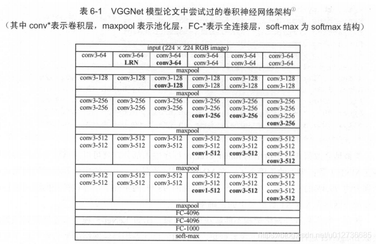
相关配置

• convX-Y：滤波器的边长为X，深度为Y
  • VGGNet中的滤波器的边长基本都为3或1
  • LeNet-5中使用了大小为55的滤波器，一般都不会超过5，但也有的设置为77，甚至11*11的
• 在滤波器的深度选择上，大部分都采用逐层递增的方式，VGG中，每经过一个池化层，滤波器的深度*2，
  • 卷积层的步长一般为2，但也有例外（使用2或3）
• 池化层配置相对简单，用的最多的是最大池化层，边长一般为2或3，步长一般为2或3

3、Inception-v3模型

已知滤波器的大小可选，但是没有先验知识帮助我们去选择其大小，所以Inception模型将不同尺寸的滤波器的滤波结果通过并联的方式结合在一起，即将得到的矩阵拼接起来。

（１）Inception结构

Inception模型会使用不同尺寸的滤波器处理矩阵，使用全0填充和步长为1的方法获得的特征图谱大小是相同的，不会影响矩阵的拼接。

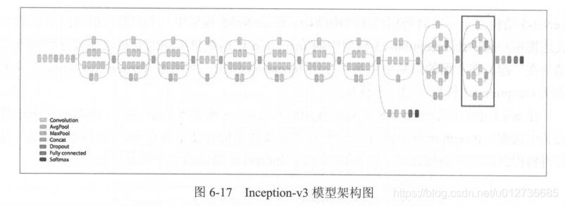
Inception-v3模型共有46层，由11个Inception模块构成，上图中方框标注的就是一个模块，Inception-v3模型有96个卷积层，直接使用上文的TensorFlow模型会非常冗长，所以此处介绍TensorFlow-Slim工具来更加简洁的实现同样结构的神经网络代码量。

• 直接使用TensorFlow原始API实现卷积层.

with tf.variable_scope(scope_name):
	weights = tf.get_variable("weights", ...)
	biases = tf.get_variable("biases", ...)
	conv = tf.nn.conv2d(...)
	relu = tf.nn.relu(tf.nn.bias_add(conv, biases))

• 使用TensorFlow-Slim实现卷积层

import tensorflow.contrib.slim as slim

tf.contrib.slim.conv2d (inputs,
            num_outputs,#[卷积核个数]
            kernel_size,#[高度，宽度]
            stride=1,#步长
            padding='SAME',#VALID）
net=slim.conv2d(input,32,[3,3])
# 可以在一行中实现一个卷积层的前向传播算法
# 第一个参数：输入节点矩阵
# 第二个参数：当前卷积层过滤器的深度
# 第三个参数：过滤器的尺寸
# 可选步长、填充、激活函数、变量命名空间等

（２）Inception模块实现

# loading the lib of slim
import tensorflow as tf

slim = tf.contrib.slim

# slim.arg_scope函数用于设置默认参数取值。
# 第一个参数：一个函数列表。该列表中函数将使用默认的参数取值
# 调用slim.conv2d(net,  320 ,  [1 , 1])函数时会自动加上 stride=1 和 padding＝’ SAME’的参数。若函数调用时指定stride，则这里默认值就补在使用。
# 作用：较少冗余的代码

# loading the lib of slim
with slim.arg_scope([slim.conv2d, slim.max_pool2d, slim.avg_pool2d], stride=1, padding='VALID):
	...
	# 此处省略Inception-v3模型中年其他网络结构而直接实现最后方框中的Inception结构。
	# 假设：输入图片经过之前的神经网络前向传播的结果保存在变量net中。
	net = 上一层的输出节点矩阵
	# 为一个 Inception 模块声明一个统一的变量命名空间。
	with tf.variable_scope('Mixed_7c'):
		# 给 Inception 模块中每一条路径声明一个命名空间。
		with tf.variable_scope('Branch_0'):
			# 实现一个过滤器边长为 1 ，深度为 320 的卷积层。
			branch_0 = slim.conv2d(net, 320, [1, 1], scope='Conv2d_0a_1x1')
		with tf.variable_scope('Branch_1'):
			branch_1 = slim.conv2d(net, 384, [1, 1], scope='Conv2d_0a_1x1')
			# tf.concat函数可以将多个矩阵拼接起来。
			# 第一个参数:拼接的维度, "3"代表了矩阵是在深度这个维度上进行拼接,如图 6-16 所示
			branch_1 = tf.concat(3, [
				# 如图 6-17 所示，此处 2 层卷积层的输入都是branch_1而不是net
				slim.conv2d(branch_1, 384, [1, 3], scope='Conv2d_0b_1x3'),
				slim.conv2d(branch_1, 384, [3, 1], scope='Conv2d_0c_3x1')])

		with tf.variable_scope('Branch_2'):
			branch_2 = slim.conv2d(net, 448, [1, 1], scope='Conv2d_0a_1x1')
			branch_2 = slim.conv2d(branch_2, 384, [3, 3], scope='Conv2d_0b_3x3')
			branch_2 = tf.concat(3, [
				slim.conv2d(branch_2, 384, [1, 3], scope='Conv2d_0c_1x3'),
				slim.conv2d(branch_2, 384, [3, 1], scope='Conv2d_0d_3x1')])

		with tf.variable_scope('Branch_3'):
			branch_3 = slim.avg_pool2d(net, [3, 3], scope='AvgPool_0a_3x3')
			branch_3 = slim.conv2d(branch_3, 192, [1, 1], scope='Conv2d_0b_1x1')
			
		# Inception 模块的最后输出是由上面 4 个计算结果拼接得到的。
		net = tf.concat(3, [branch_0, branch_1, branch_2, branch_3])
	

五、ＣＮＮ迁移学习

1、迁移学习介绍

目标：为了解决标注数据和训练时间的问题。（很难收集到非常多的标注数据；要训练一个复杂的卷积神经网络需要几天甚至几周的时间 。）
不足：一般来说，在数据量足够的情况下，迁移学习的效果不如完全重新训练。但是迁移学习所需要的训练时间和训练样本数要远远小于训练完整的模型 。

迁移学习：将一个问题上训练好的模型通过简单的调整使其适用于一个新的问题 。

实例：利用 ImageNet 数据集上训练好的 Inception-v3 模型来解决一个新的图像分类问题 。 根据论文 DeCAF: A Deep Convolutional Activation Feature for Generic Visual Recognition 中的结论，可以保留训练好的 Inception-v3 模型中所有卷积层的参数，只是替换最后一层全连接层。 在最后这一层全连接层之前的网络层称之为瓶颈层（ bottleneck ）。

2、TF实现迁移学习

（１）获取数据集

wget http://download.tensorflow.org/example_images/flower_photos.tgz
tar xzf flower_photos.tgz

文件夹包含了 5 个子文件夹 ， 每一个子文件夹的名称为一种花的名称，代表了不同的类别 。平均每一种花有 734 张图片，每一张图片都是 RGB 色彩模式的，大小也不相同。

（２）数据预处理

将原始的图像数据整理成模型需要的输入数据。
==》将所有的图片数据划分成训练、 验证和测试 3 个数据集；图像转换为2992993的数字矩阵。

#-*-coding:utf-8-*-

import tensorflow as tf
import glob
import os.path
import numpy as np
from tensorflow.contrib.slim import slim
from tensorflow.python.platform import gfile

# 原始输入数据的目录
INPUT_DATA = './datasets/flower_photos'
# 输出文件地址。将整理后的图片数据通过 numpy 的格式保存。
OUTPUT_FILE = './datasets/flower_processed_data.npy'

# 测试数据和验证数据比例。
VALIDATION_PERCENTAGE = 10
TEST_PERCENTAGE = 10

def create_image_lists(sess, testing_percentage, valiation_percentage):
	sub_dirs = [x[0] for x in os.walk(INPUT_DATA)]
	is_root_dir = True

	# 初始化各个数据集
	training_images = []
	training_labels = []
	testing_images = []
	testing_labels = []
	valiation_images = []
	valiation_labels = []
	current_label = 0
	count = 0

	# 读取所有的子目录。
	for sub_dir in sub_dirs:
		if is_root_dir:
			is_root_dir = False
			continue
		# 获取一个子目录中所有的图片文件。
		extensions = ['jpg']
		file_list = []
		dir_name = os.path.basename(sub_dir)
		for extension in extensions:
			file_glob = os.path.join(INPUT_DATA, dir_name, '*.'+extension)
			file_list.extend(glob.glob(file_glob))
			if not file_list: continue

			# 处理图片数据。
			for file_name in file_list:
				# 读取并解析图片，将图片转化为299×299以便inception-v3模型来处理。
				image_raw_data = gfile.FastGFile(file_name, 'rb').read()
				image = tf.image.decode_jpeg(image_raw_data)
				if image.dtype != tf.float32:
					image = tf.image.convert_image_dtype(image, dtype=tf.float32)
				image = tf.image.resize_images(image, [229, 229])
				image_value = sess.run(image)

				# 随机划分数据集
				chance = np.random.randint(100)
				if chance < valiation_percentage:
					valiation_images.append(image_value)
					valiation_labels.append(current_label)
				elif chance < (testing_percentage + valiation_percentage):
					testing_images.append(image_value)
					testing_labels.append(current_label)
				else:
					training_images.append(image_value)
					training_labels.append(current_label)
				count = count + 1
				print('count: ', count)
			current_label += 1

	# 将训练数据随机打乱以获得更好的训练效果。
	state = np.random.get_state()
	np.random.shuffle(training_images)
	np.random.set_state(state)
	np.random.shuffle(training_labels)
	return np.asarray([training_images, training_labels,
					   valiation_images,valiation_labels,
					   testing_images, testing_labels])

# 数据整理主函数。
def main():
	with tf.Session() as sess:
		processed_data = create_image_lists(sess, TEST_PERCENTAGE, VALIDATION_PERCENTAGE)
		np.save(OUTPUT_FILE, processed_data)

if __name__ == '__main__':
	main()

（３）获取预训练模型

wget https://storage.googleapis.com/download.tensorflow.org/models/inception_v3_2016_08_28.tar.gz
tar xzf inception_v3_2016_08_28.tar.gz

（４）迁移学习代码实现

INPUT_DATA = './datasets/flower_photos/flower_processed_data.npy'
TRAIN_FILE = './model/transfer'
CKPT_FILE = './model/inception_v3_2016_08_28/inception_v3.ckpt'

LEARNING_RATE = 0.0001
STEPS = 300
BATCH = 32
N_CLASSES = 5

# 不需要从预训练好的模型中加载的参数。（最后的全连接层）
CHECKPOINT_EXCLUDE_SCOPES = 'InceptionV3/Logits, InceptionV3/AuxLogits'
# 需要训练的网络层参数名称，在fine-tuning过程中就是最后的全连接层
TRAINABLE_SCOPES='InceptionV3/Logits, InceptionV3/AuxLogits'

# 获取所有需要从预训练模型中加载的参数
def get_tuned_variables():
	exclusions = [scope.strip() for scope in CHECKPOINT_EXCLUDE_SCOPES.split(',')]

	variables_to_restore = []
	# 枚举inception-v3模型中所有的参数，然后判断是否满要从加载列表中移除。
	for var in slim.get_model_variables():
		excluded = False
		for extension in exclusions:
			if var.op.name.startswith(extension):
				excluded = True
				break
		if not excluded:
			variables_to_restore.append(var)
	return variables_to_restore

# 获取所有需要训练的变量列表。
def get_trainable_variables():
	scopes = [scope.strip() for scope in TRAINABLE_SCOPES.split(',')]
	variables_to_train = []
	# 枚举所有需要训练的参数前缀，并通过这些前缀找到所有的参
	for scope in scopes:
		variables = tf.get_collection(tf.GraphKeys.TRAINABLE_VARIABLES, scope)
		variables_to_train.extend(variables)
	return variables_to_train

def main():
	# 加载预处理好的数据。
	processed_data = np.load(INPUT_DATA)
	training_images = processed_data[0]
	n_training_example = len(training_images)
	training_labels = processed_data[1]
	valiation_images = processed_data[2]
	valiation_labels = processed_data[3]
	testing_images = processed_data[4]
	testing_labels = processed_data[5]
	print("%d training examples, %d valiation examples and %d testing examples."
			% (n_training_example, len(valiation_labels), len(testing_labels)))

	# 定义inception-v3的输入，images为输入图片，labels为每一张图片对应的标签。
	images = tf.placeholder(tf.float32, [None, 299, 299, 3], name='input_image')
	labels = tf.placeholder(tf.int64, [None], name='labels')

	# 定义 inception-v3 模型。
	# 预训练模型只有模型参数取值，所以代码中需定义inception-v3的模型结构。
	# 虽然理论上需要区分训练和测试中使用的模型，也就是说在测试时应该使用 is training=False，
	# 但是因为预先训练好的 inception-v3 模型中使用的 batch normalization 
	# 参数与新的数据会有差异，导致结果很差，所以这里直接使用同一个模型来进行测试。
	with slim.arg_scope(inception_v3.inception_v3_arg_scope()):
		logits, _ = inception_v3.inception_v3(images, num_classes=N_CLASSES)
	# 获取需要训练的变量。
	trainable_variables = get_trainable_variables()
	# 定义交叉熵损失。注意在模型定义的时候己经将正则化损失加入损失集合了。
	tf.losses.softmax_cross_entropy(tf.one_hot(labels, N_CLASSES), logits, weights=1.0)
	# 定义训练过程。这里 minimize 的过程中指定了需要优化的变量集合。
	train_step = tf.train.RMSPropOptimizer(LEARNING_RATE).minimize(tf.losses.get_total_loss())

	# accuracy
	with tf.name_scope('evaluation'):
		correct_prediction = tf.equal(tf.argmax(logits, 1), labels)
		evaluation_step = tf.reduce_mean(tf.cast(correct_prediction, tf.float32))
	# 定义加载模型的函数。
	load_fn = slim.assign_from_checkpoint_fn(
		CKPT_FILE,
		get_tuned_variables(),
		ignore_missing_vars=True)

	# 定义保存新的训练好的模型的函数
	saver = tf.train.Saver()
	with tf.Session() as sess:
		# 初始化没有加载进来的变量。注意这个过程一定要在模型加载之前，
		# 否则初始化过程会将已经加载好的变量重新赋值
		init = tf.global_variables_initializer()
		sess.run(init)

		# 加载预训练模型
		print("Loading tuned variables from %s" % CKPT_FILE)
		load_fn(sess)

		start = 0
		end = BATCH
		for i in range(STEPS):
			# 运行训练过程，这里不会更新全部的参数，只会更新指定的部分参数。
			sess.run(train_step, feed_dict={
				images:training_images[start:end],
				labels:training_labels[start:end] })

			# 输出日志
			if i % 30 == 0 or i + 1 == STEPS:
				saver.save(sess, TRAIN_FILE, global_step = i)
				valiation_accuracy = sess.run(evaluation_step,feed_dict={
					images:valiation_images,
					labels:valiation_labels })
				print("Step %d: Validation accuracy = %.1f%%" % (i, valiation_accuracy*100.0))

			# 因为在数据预处理时做了打乱数据的操作，所以这里需顺序使用训练数据就好。
			start = end
			if start == n_training_example:
				start = 0

			end = start + batch
			if end > n_training_example:
				end = n_training_example

		# testing
		test_accuracy = sess.run(evaluation_step, feed_dict={
			images:testing_images, labels:testing_labels })
		print('Final test accuracy = %.1f%%' % (test_accuracy * 100))

if __name__ == '__main__':
	main()

输出结果

Step 0: Validation accuracy = 26.4%
Step 30: Validation accuracy = 29.5%
Step 60: Validation accuracy = 43.5%
Step 90: Validation accuracy = 77.7%
Step 120: Validation accuracy = 89.6%
Step 150: Validation accuracy = 90.2%
Step 180: Validation accuracy = 94.8%
Step 210: Validation accuracy = 94.3%
Step 240: Validation accuracy = 95.3%
Step 270: Validation accuracy = 95.3%
Step 299: Validation accuracy = 93.8%
2019-03-21 10:37:45.608084: W tensorflow/core/common_runtime/bfc_allocator.cc:219] Allocator (GPU_0_bfc) ran out of memory trying to allocate 3.67GiB. The caller indicates that this is not a failure, but may mean that there could be performance gains if more memory were available.
2019-03-21 10:37:46.101814: W tensorflow/core/common_runtime/bfc_allocator.cc:219] Allocator (GPU_0_bfc) ran out of memory trying to allocate 3.67GiB. The caller indicates that this is not a failure, but may mean that there could be performance gains if more memory were available.
Final test accuracy = 92.0%