版权声明:本文为博主原创文章,未经博主允许不得转载。 https://blog.csdn.net/SunChao3555/article/details/88377681
import numpy as np
import pandas as pd
import matplotlib.pyplot as plt
import pylab,os
from pandas import DataFrame, Series
from keras import models, layers, optimizers, losses, metrics
from keras.utils.np_utils import to_categorical
from keras.preprocessing.image import ImageDataGenerator
#更靠近底部的层是指在定义模型时先添加到模型中的层,而更靠近顶部的层则是后添加到模型中的层
'''
通过进一步使用正则化方法以及调节网络参数(比如每个卷积
层的过滤器个数或网络中的层数),你可以得到更高的精度,可以达到86%或87%。但只靠从头开始训练自己的卷
积神经网络,再想提高精度
就十分困难,因为可用的数据太少。想要在这个问题上进一步提高精度,
下一步需要使用预训练的模型
预训练网络(pretrained network)是一个保存好的网络,之前
已在大型数据集(通常是大规模图像分类任务)上训练好。如果
这个原始数据集足够大且足够通用,那么预训练网络学到的特征
的空间层次结构可以有效地作为视觉世界的通用模型,因此这些
特征可用于各种不同的计算机视觉问题,即使这些新问题涉及的
类别和原始任务完全不同
第一次遇到这种奇怪的模型名称——VGG、ResNet、Inception、Inception-ResNet、Xception 等。 你会
习惯这些名称的,因为如果你一直用深度学习做计算机视觉的话,它们会频繁出现.
预训练网络有两种方法:特征提取和微调模型
'''
#特征提取:使用之前网络学到的表示来从新样本中提取出有用的特征。然后将这些特征输入一个新的分类器,从头开始训练。
#将VGG16卷积实例化
from keras.applications import VGG16
conv_base=VGG16(
weights='imagenet',#指定模型初始化的权重检查点
include_top=False,#指定模型最后是否包含密集连接分类器(它默认对应于ImageNet的1000个类别。因
为我们打算使用自己的密集连接分类器(只有 两个类别:cat 和 dog),所以不需要包含它)
input_shape=(150,150,3))#是输入到网络中的图像张量的形状。这个参数完全是可选的,如果不传入这
个参数,那么网络能够处理任意形状的输入
print(conv_base.summary())
#可以看到卷积基最终的输出的特征图形状为(None, 4, 4, 512)。我们在这个特征上添加一个密集连接分类
器。
'''
接下来,下一步有两种方法可供选择
1.在你的数据集上运行卷积基,将输出保存成硬盘中的Numpy数组
然后用这个数据作 为输入,输入到独立的密集连接分类器中(与本第
一部分介绍的分类器类似)。这种方法速度快,计算代价低,因为对于
每个输入图像只需运行一次卷积基,而卷积基是目前流程中计算代价最
高的。但出于同样的原因,这种方法不允许你使用数据增强。
2.在顶部添加 Dense 层来扩展已有模型(即 conv_base),并在
输入数据上端到端地运行整个模型。这样你可以使用数据增强,因为每
个输入图像进入模型时都会经过卷积基。但出于同样的原因,这种方法
的计算代价比第一种要高很多。
'''
#1.不使用数据增强的快速特征提取
#-----------------------------------------------------
#-----------------------------------------------------
#使用预训练的卷积基提取特征
base_dir='F:/dogs-vs-cats/cats_and_dogs_small'
train_dir = os.path.join(base_dir, 'train')
validation_dir = os.path.join(base_dir, 'validation')
test_dir = os.path.join(base_dir, 'test')
datagen=ImageDataGenerator(rescale=1./255)
batch_size=20
def extract_features(directory,sample_count):
features=np.zeros(shape=(sample_count,4,4,512))
labels=np.zeros(shape=(sample_count))
generator=datagen.flow_from_directory(
directory,
target_size=(150,150),
batch_size=batch_size,
class_mode='binary')
i=0
for input_batch,labels_batch in generator:
features_batch=conv_base.predict(input_batch)#从图像中提取特征
features[i*batch_size :(i+1)*batch_size]=features_batch#按batch_size将特征/标签填充到numpy数组
labels[i*batch_size :(i+1)*batch_size]=labels_batch
i+=1
if i*batch_size>=sample_count:#生成器终止条件
break
return features,labels
#下面定义并训练全连接分类器并添加dropout正则化
def build_fit_model1(train_features,validation_features,test_features,train_labels,validation_labels):
model = models.Sequential()
model.add(layers.Dense(256, activation='relu', input_dim=4 * 4 * 512))
model.add(layers.Dropout(0.5))
model.add(layers.Dense(1, activation='sigmoid'))
model.compile(
optimizer=optimizers.RMSprop(lr=2e-5),
loss='binary_crossentropy',
metrics=['acc'])
train_features, train_labels = extract_features(train_dir, 2000)
validation_features, validation_labels = extract_features(validation_dir, 1000)
test_features, test_labels = extract_features(test_dir, 1000)
# 经过上述操作得到的特征形状为(samples,4,4,512)。将其输入到全连接层,需要首先展平为(samples,4*4*512)
train_features = np.reshape(train_features, (2000, 4 * 4 * 512))
validation_features = np.reshape(validation_features, (1000, 4 * 4 * 512))
test_features = np.reshape(test_features, (1000, 4 * 4 * 512))
history = model.fit(
train_features,
train_labels,
epochs=30,
batch_size=20,
validation_data=(validation_features, validation_labels))
return history
#---------------------------------------------------------
#---------------------------------------------------------
def acc_loss_plot(history):
fig=plt.figure()
ax1=fig.add_subplot(2,1,1)
acc = history.history['acc']
val_acc = history.history['val_acc']
loss = history.history['loss']
val_loss = history.history['val_loss']
epochs = range(1, len(acc) + 1)
ax1.plot(epochs, acc, 'bo', label='Training acc')
ax1.plot(epochs, val_acc, 'b', label='Validation acc')
ax1.set_title('Training and validation accuracy')
ax2=fig.add_subplot(2,1,2)
ax2.plot(epochs, loss, 'bo', label='Training loss')
ax2.plot(epochs, val_loss, 'b', label='Validation loss')
ax2.set_title('Training and validation loss')
plt.legend()
plt.tight_layout()
plt.show()
# history=build_fit_model1(train_features,validation_features,test_features)
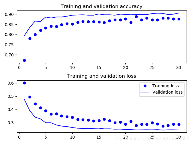
# acc_loss_plot(history)#验证精度达到了90%
#虽然 dropout 比率相当大,但模型几乎从一开始就过拟合。这是因为本方法没有使用数据增强,而数据增强对防止小型图像数据集的过拟合非常重要
#2.使用数据增强的特征提取:扩展conv_base模型,然后在输入数据上端到端地运行模型(速度更慢,计算代价更高)
def build_model2():
model=models.Sequential()
model.add(conv_base)
model.add(layers.Flatten())
model.add(layers.Dense(256, activation='relu', input_dim=4 * 4 * 512))
# model.add(layers.Dropout(0.5))
model.add(layers.Dense(1, activation='sigmoid'))
print(model.summary())#可以看出VCG16的卷积基有14714688个参数,因此在编译和训练模型之前一定要‘冻结’卷积基。
'''
#冻结(freeze)一个或多个层是指在训练过程中保持其权重不变
如果不这么做,那么卷积基之前学到的表示将会在训练过程
中被修改。 因为其上添加的 Dense 层是随机初始化的,所以
非常大的权重更新将会在网络中传播,对之前学到的表示造成很
大破坏
#在 Keras 中,冻结网络的方法是将其 trainable 属性设为 False
'''
return model
def freeze_all():
print('This is the number of trainable weights before freezing the conv base:', len(model.trainable_weights))
conv_base.trainable = False
print('after freezing the conv base:', len(model.trainable_weights))
# 设置之后,只有添加的两个Dense层的权重才会被训练。
# 总共有 4 个权重张量,每层2 个(主权重矩阵和偏置向量)。
# 注意,为了让这些修改生效,你必须在编译模型前设置
def compile_fit_model2(model,train_dir,validation_dir):
# freeze_all()
freeze_option()#微调模型[见后续]
#使用和之前数据增强例子的相同设置
train_datagen = ImageDataGenerator(
rescale=1. / 255,
rotation_range=40,
width_shift_range=0.2,
height_shift_range=0.2,
shear_range=0.2,
zoom_range=0.2,
horizontal_flip=True,
fill_mode='nearest')
train_generator = train_datagen.flow_from_directory(
train_dir,
target_size = (150, 150),
batch_size = 20,
class_mode = 'binary')
validation_generator = test_datagen.flow_from_directory(
validation_dir,
target_size = (150, 150),
batch_size = 20,
class_mode = 'binary')
model.compile(
loss='binary_crossentropy',
optimizer=optimizers.RMSprop(lr=1e-5),
metrics=['acc'])
history = model.fit_generator(
train_generator,
steps_per_epoch=100,
# epochs=30,
epochs=100,
validation_data=validation_generator,
validation_steps=50)
return history
# model=build_model2()
# history=compile_fit_model2(model,train_dir,validation_dir)
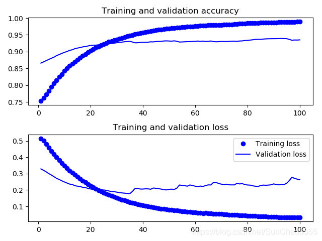
# acc_loss_plot(history)#发现数据精确度在90%左右(或许轮数不够个人在设置epochs=30精确度并没有达到作者所说的验证精度96%,但确实没有发生过拟合)
#微调模型
'''
对于用于特征提取的冻结的模型基,微调是指将其顶部的几层“解冻”,并将这解冻的几层和新增加的部分(本
例中是全连接分类器)联合训练
微调:略微调整了所复用模型中更加抽象的表示,以便让这些表示与手头的问题更加相关
#前面说过,冻结 VGG16 的卷积基是为了能够在上面训练一个随机初始化的分类器。同理, 只有上面的分类器
已经训练好了,才能微调卷积基的顶部几层。如果分类器没有训练好,那么训练期间通过网络传播的误差信号会特别大,微调的几层之前学到的表示都会被破坏。因此, 微调网络的步骤如下。
(1) 在已经训练好的基网络(base network)上添加自定义网络
(2) 冻结基网络。
(3) 训练所添加的部分。
(4) 解冻基网络的一些层。
(5) 联合训练解冻的这些层和添加的部分。
在做特征提取时已经完成了前三个步骤。我们继续进行第四步:
先解冻 conv_base,然后冻结其中的部分层。
'''
# model=build_model2()#可以看到VGG16共由5个block组成。
'''
微调最后三个卷积层,即block5_...,那么直到block4_pool的所有层都应该被冻结,而block5_conv1、block5_conv2 和 block5_conv3 三层应该是可训练的。
为什么不微调更多层?为什么不微调整个卷积基?你当然可以这么做,但需要考虑以下几点
1.卷积基中更靠底部的层编码的是更加通用的可复用特征,而更靠顶部的层编码的是更专 业化的特征。微
调这些更专业化的特征更加有用,因为它们需要在你的新问题上改变用途。微调更靠底部的层,得到的回报会
更少
2.训练的参数越多,过拟合的风险越大。卷积基有1500万个参数所以在你的小型数据 集上训练这么多参数是有风险的。
因此,在这种情况下,一个好策略是仅微调卷积基最后的两三层
'''
#冻结直到某一层的所有层
def freeze_option():
conv_base.trainable=True
set_trainable=False
for layer in conv_base.layers:
if layer.name=='block5_conv1':
set_trainable=True
if set_trainable:
layer.trainable=True
else:
layer.trainable=False
#微调模型
#们将使用学习率非常小的 RMSProp 优化器来实现。之所以让学习率很小,是因为对于微调的三层表示,我们希望其变化范围不要太大。太大的权重更新可能会破坏这些表示。
model=build_model2()
history=compile_fit_model2(model,train_dir,validation_dir)
def smooth_curve(points, factor=0.9):#将每个数据点替换为前面数据点的指数移动平均值,以得到光滑的曲线
smoothed_points = []
for point in points:
if smoothed_points:
previous = smoothed_points[-1]
smoothed_points.append(previous * factor + point * (1 - factor))
else:
smoothed_points.append(point)
return smoothed_points
def acc_loss_smooth_plot(history):
fig = plt.figure()
ax1 = fig.add_subplot(2, 1, 1)
acc = history.history['acc']
val_acc = history.history['val_acc']
loss = history.history['loss']
val_loss = history.history['val_loss']
epochs = range(1, len(acc) + 1)
ax1.plot(epochs, smooth_curve(acc), 'bo', label='Training acc')
ax1.plot(epochs, smooth_curve(val_acc), 'b', label='Validation acc')
ax1.set_title('Training and validation accuracy')
ax2 = fig.add_subplot(2, 1, 2)
ax2.plot(epochs, smooth_curve(loss), 'bo', label='Training loss')
ax2.plot(epochs, smooth_curve(val_loss), 'b', label='Validation loss')
ax2.set_title('Training and validation loss')
plt.legend()
plt.tight_layout()
plt.show()
acc_loss_smooth_plot(history)#模型验证精度达到95%左右
#注意:从损失曲线上看不出与之前相比有任何真正的提高(实际上还在变差)。你可能感到奇怪,如果损失没
有降低,那么精度怎么能保持稳定或提高呢?答案很简单:图中展示的是逐 点pointwise)损失值的平均值,
但影响精度的是损失值的分布,而不是平均值,因为精度是 模型预测的类别概率的二进制阈值。即使从平均损
失中无法看出,但模型也仍然可能在改进
#在测试集上评估模型
test_datagen = ImageDataGenerator(rescale=1. / 255)
test_generator=test_datagen.flow_from_directory(
test_dir,
target_size=(150,150),
batch_size=20,
class_mode='binary',
)
test_loss,test_acc=model.evaluate(test_generator,steps=50)
print('test_acc:',test_acc)
使用預训练网络进行特征提取操作后的accuracy和loss图示
使用模型微调后的图示
'''
卷积神经网络是用于计算机视觉任务的最佳机器学习模型。即使在非常小的数据集上也可以从头开始训练一个卷积神经网络,而且得到的结果还不错
在小型数据集上的主要问题是过拟合。在处理图像数据时,数据增强是一种降低过拟合的强大方法
利用特征提取,可以很容易将现有的卷积神经网络复用于新的数据集。对于小型图像数据集,这是一种很有价值的方法
作为特征提取的补充,你还可以使用微调,将现有模型之前学到的一些数据表示应用于新问题。这种方法可以进一步提高模型性能
'''