TensorFlow2.0教程-回归

版权声明：本文为博主原创文章，未经博主允许不得转载。 https://blog.csdn.net/qq_31456593/article/details/88778647

TensorFlow2.0教程-回归

Tensorflow 2.0 教程持续更新 ：https://blog.csdn.net/qq_31456593/article/details/88606284

完整tensorflow2.0教程代码请看tensorflow2.0：中文教程tensorflow2_tutorials_chinese(欢迎star)

入门教程：
TensorFlow 2.0 教程- Keras 快速入门
TensorFlow 2.0 教程-keras 函数api
TensorFlow 2.0 教程-使用keras训练模型
TensorFlow 2.0 教程-用keras构建自己的网络层
TensorFlow 2.0 教程-keras模型保存和序列化

在回归问题中，我们的目标是预测连续值的输出，如价格或概率。
我们采用了经典的Auto MPG数据集，并建立了一个模型来预测20世纪70年代末和80年代初汽车的燃油效率。 为此，我们将为该模型提供该时段内许多汽车的描述。 此描述包括以下属性：气缸，排量，马力和重量。

1.Auto MPG数据集

获取数据

dataset_path = keras.utils.get_file('auto-mpg.data',
                                   'https://archive.ics.uci.edu/ml/machine-learning-databases/auto-mpg/auto-mpg.data')

print(dataset_path)

Downloading data from https://archive.ics.uci.edu/ml/machine-learning-databases/auto-mpg/auto-mpg.data
32768/30286 [================================] - 1s 25us/step
/home/czy/.keras/datasets/auto-mpg.data

使用pandas读取数据

column_names = ['MPG','Cylinders','Displacement','Horsepower','Weight',
                'Acceleration', 'Model Year', 'Origin'] 
raw_dataset = pd.read_csv(dataset_path, names=column_names,
                         na_values='?', comment='\t',
                         sep=' ', skipinitialspace=True)
dataset = raw_dataset.copy()
dataset.tail()

	MPG	Cylinders	Displacement	Horsepower	Weight	Acceleration	Model Year	Origin
393	27.0	4	140.0	86.0	2790.0	15.6	82	1
394	44.0	4	97.0	52.0	2130.0	24.6	82	2
395	32.0	4	135.0	84.0	2295.0	11.6	82	1
396	28.0	4	120.0	79.0	2625.0	18.6	82	1
397	31.0	4	119.0	82.0	2720.0	19.4	82	1

2.数据预处理

清洗数据

print(dataset.isna().sum())
dataset = dataset.dropna()
origin = dataset.pop('Origin')
dataset['USA'] = (origin == 1)*1.0
dataset['Europe'] = (origin == 2)*1.0
dataset['Japan'] = (origin == 3)*1.0
dataset.tail()

MPG             0
Cylinders       0
Displacement    0
Horsepower      6
Weight          0
Acceleration    0
Model Year      0
Origin          0
dtype: int64

	MPG	Cylinders	Displacement	Horsepower	Weight	Acceleration	Model Year	USA	Europe	Japan
393	27.0	4	140.0	86.0	2790.0	15.6	82	1.0	0.0	0.0
394	44.0	4	97.0	52.0	2130.0	24.6	82	0.0	1.0	0.0
395	32.0	4	135.0	84.0	2295.0	11.6	82	1.0	0.0	0.0
396	28.0	4	120.0	79.0	2625.0	18.6	82	1.0	0.0	0.0
397	31.0	4	119.0	82.0	2720.0	19.4	82	1.0	0.0	0.0

划分训练集和测试集

train_dataset = dataset.sample(frac=0.8,random_state=0)
test_dataset = dataset.drop(train_dataset.index)

检测数据

观察训练集中几对列的联合分布。

sns.pairplot(train_dataset[["MPG", "Cylinders", "Displacement", "Weight"]], diag_kind="kde")

<seaborn.axisgrid.PairGrid at 0x7f934072fe10>

整体统计数据：

train_stats = train_dataset.describe()
train_stats.pop("MPG")
train_stats = train_stats.transpose()
train_stats

	count	mean	std	min	25%	50%	75%	max
Cylinders	314.0	5.477707	1.699788	3.0	4.00	4.0	8.00	8.0
Displacement	314.0	195.318471	104.331589	68.0	105.50	151.0	265.75	455.0
Horsepower	314.0	104.869427	38.096214	46.0	76.25	94.5	128.00	225.0
Weight	314.0	2990.251592	843.898596	1649.0	2256.50	2822.5	3608.00	5140.0
Acceleration	314.0	15.559236	2.789230	8.0	13.80	15.5	17.20	24.8
Model Year	314.0	75.898089	3.675642	70.0	73.00	76.0	79.00	82.0
USA	314.0	0.624204	0.485101	0.0	0.00	1.0	1.00	1.0
Europe	314.0	0.178344	0.383413	0.0	0.00	0.0	0.00	1.0
Japan	314.0	0.197452	0.398712	0.0	0.00	0.0	0.00	1.0

取出标签

train_labels = train_dataset.pop('MPG')
test_labels = test_dataset.pop('MPG')

标准化数据

最好使用不同比例和范围的特征进行标准化。 虽然模型可能在没有特征归一化的情况下收敛，但它使训练更加困难，并且它使得结果模型依赖于输入中使用的单位的选择。

def norm(x):
    return (x - train_stats['mean']) / train_stats['std']
normed_train_data = norm(train_dataset)
normed_test_data = norm(test_dataset)

3.构建模型

def build_model():
    model = keras.Sequential([
        layers.Dense(64, activation='relu', input_shape=[len(train_dataset.keys())]),
        layers.Dense(64, activation='relu'),
        layers.Dense(1)
    ])
    
    optimizer = tf.keras.optimizers.RMSprop(0.001)
    model.compile(loss='mse',
                 optimizer=optimizer,
                 metrics=['mae', 'mse'])
    return model

model = build_model()
model.summary()

Model: "sequential"
_________________________________________________________________
Layer (type)                 Output Shape              Param #   
=================================================================
dense (Dense)                (None, 64)                640       
_________________________________________________________________
dense_1 (Dense)              (None, 64)                4160      
_________________________________________________________________
dense_2 (Dense)              (None, 1)                 65        
=================================================================
Total params: 4,865
Trainable params: 4,865
Non-trainable params: 0
_________________________________________________________________

example_batch = normed_train_data[:10]
example_result = model.predict(example_batch)
example_result

array([[0.18062565],
       [0.1714489 ],
       [0.22555563],
       [0.29366603],
       [0.69764495],
       [0.08851457],
       [0.6851174 ],
       [0.32245407],
       [0.02959149],
       [0.38945067]], dtype=float32)

4.训练模型

class PrintDot(keras.callbacks.Callback):
    def on_epoch_end(self, epoch, logs):
        if epoch % 100 == 0: print('')
        print('.', end='')

EPOCHS = 1000

history = model.fit(
  normed_train_data, train_labels,
  epochs=EPOCHS, validation_split = 0.2, verbose=0,
  callbacks=[PrintDot()])

....................................................................................................
....................................................................................................
....................................................................................................
....................................................................................................
....................................................................................................
....................................................................................................
....................................................................................................
....................................................................................................
....................................................................................................
....................................................................................................

查看训练记录

hist = pd.DataFrame(history.history)
hist['epoch'] = history.epoch
hist.tail()

	loss	mae	mse	val_loss	val_mae	val_mse	epoch
995	2.191127	0.940755	2.191127	10.422818	2.594117	10.422818	995
996	2.113679	0.903680	2.113679	10.723925	2.631320	10.723926	996
997	2.517261	0.989557	2.517261	9.497868	2.379198	9.497869	997
998	2.250272	0.931618	2.250272	11.017041	2.658538	11.017041	998
999	1.976393	0.853547	1.976393	9.890977	2.491739	9.890977	999

def plot_history(history):
    hist = pd.DataFrame(history.history)
    hist['epoch'] = history.epoch

    plt.figure()
    plt.xlabel('Epoch')
    plt.ylabel('Mean Abs Error [MPG]')
    plt.plot(hist['epoch'], hist['mae'],
           label='Train Error')
    plt.plot(hist['epoch'], hist['val_mae'],
           label = 'Val Error')
    plt.ylim([0,5])
    plt.legend()

    plt.figure()
    plt.xlabel('Epoch')
    plt.ylabel('Mean Square Error [$MPG^2$]')
    plt.plot(hist['epoch'], hist['mse'],
           label='Train Error')
    plt.plot(hist['epoch'], hist['val_mse'],
           label = 'Val Error')
    plt.ylim([0,20])
    plt.legend()
    plt.show()


plot_history(history)

使用early stop

model = build_model()


early_stop = keras.callbacks.EarlyStopping(monitor='val_loss', patience=10)

history = model.fit(normed_train_data, train_labels, epochs=EPOCHS,
                    validation_split = 0.2, verbose=0, callbacks=[early_stop, PrintDot()])

plot_history(history)

..........................................................

测试

loss, mae, mse = model.evaluate(normed_test_data, test_labels, verbose=0)

print("Testing set Mean Abs Error: {:5.2f} MPG".format(mae))

Testing set Mean Abs Error:  1.85 MPG

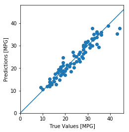
5.预测

test_predictions = model.predict(normed_test_data).flatten()
plt.scatter(test_labels, test_predictions)
plt.xlabel('True Values [MPG]')
plt.ylabel('Predictions [MPG]')
plt.axis('equal')
plt.axis('square')
plt.xlim([0,plt.xlim()[1]])
plt.ylim([0,plt.ylim()[1]])
_ = plt.plot([-100, 100], [-100, 100])

error = test_predictions - test_labels
plt.hist(error, bins = 25)
plt.xlabel("Prediction Error [MPG]")
_ = plt.ylabel("Count")