Tutorial :DEEP LEARNING WITH PYTORCH: A 60 MINUTE BLITZ
PyTorch是一个基于python的科学计算包,主要针对两类人群:
- 作为NumPy的替代品,可以利用GPU的性能进行计算
- 作为一个高灵活性、速度快的深度学习平台
目录
Getting Started:Tensors,Operations
NumPy Bridge:Converting a Torch Tensor to a NumPy Array,Converting NumPy Array to Torch Tensor
AUTOGRAD: AUTOMATIC DIFFERENTIATION
Define the network;Loss Function;Backprop;Update the weights
1. Loading and normalizing CIFAR10
2. Define a Convolutional Neural Network
3. Define a Loss function and optimizer
5. Test the network on the test data
Training on GPU;Training on multiple GPUs;Where do I go next?
Imports and parameters;Dummy DataSet;Simple Model;Create Model and DataParallel;Run the Model
WHAT IS PYTORCH?
Getting Started
Tensors
Tensors are similar to NumPy’s ndarrays, with the addition being that Tensors can also be used on a GPU to accelerate computing.
from __future__ import print_function
import torch
Construct a 5x3 matrix, uninitialized:
x = torch.empty(5, 3)
print(x)
Out:
tensor([[-7.7749e-18,  4.5649e-41, -1.6017e-15],
        [ 4.5649e-41,  0.0000e+00,  1.4013e-45],
        [ 0.0000e+00,  0.0000e+00,  0.0000e+00],
        [ 0.0000e+00,  0.0000e+00,  0.0000e+00],
        [ 0.0000e+00,  0.0000e+00,  0.0000e+00]])
Construct a randomly initialized matrix:
x = torch.rand(5, 3)
print(x)
Out:
tensor([[0.9376, 0.8087, 0.1564],
        [0.6768, 0.2201, 0.6317],
        [0.0075, 0.7946, 0.1698],
        [0.8816, 0.2601, 0.2858],
        [0.4335, 0.8111, 0.4825]])
Construct a matrix filled zeros and of dtype long:
x = torch.zeros(5, 3, dtype=torch.long)
print(x)
Out:
tensor([[0, 0, 0],
        [0, 0, 0],
        [0, 0, 0],
        [0, 0, 0],
        [0, 0, 0]])
Construct a tensor directly from data:
x = torch.tensor([5.5, 3])
print(x)
Out:
tensor([5.5000, 3.0000])
or create a tensor based on an existing tensor. These methods will reuse properties of the input tensor, e.g. dtype, unless new values are provided by user
x = x.new_ones(5, 3, dtype=torch.double)      # new_* methods take in sizes
print(x)

x = torch.randn_like(x, dtype=torch.float)    # override dtype!
print(x)                                      # result has the same size
Out:
tensor([[1., 1., 1.],
        [1., 1., 1.],
        [1., 1., 1.],
        [1., 1., 1.],
        [1., 1., 1.]], dtype=torch.float64)
tensor([[-1.6285, -0.6166, -0.6149],
        [ 0.1568,  0.1322,  0.4867],
        [ 0.2416, -0.1859, -2.9161],
        [-0.0097,  2.4822,  0.0418],
        [-1.1505, -0.4131, -0.5941]])
Get its size:
print(x.size())Out:
torch.Size([5, 3])
NOTE
torch.Size is in fact a tuple, so it supports all tuple operations.
Operations
There are multiple syntaxes for operations. In the following example, we will take a look at the addition operation.
Addition: syntax 1
y = torch.rand(5, 3)
print(x + y)
Out:
tensor([[-0.7917,  0.2000,  0.3005],
        [ 0.2331,  0.5763,  1.4071],
        [ 0.4486, -0.0042, -2.0666],
        [ 0.7748,  2.9549,  0.9221],
        [-0.4646, -0.0807, -0.0748]])
Addition: syntax 2
print(torch.add(x, y))Out:
tensor([[-0.7917,  0.2000,  0.3005],
        [ 0.2331,  0.5763,  1.4071],
        [ 0.4486, -0.0042, -2.0666],
        [ 0.7748,  2.9549,  0.9221],
        [-0.4646, -0.0807, -0.0748]])
Addition: providing an output tensor as argument
result = torch.empty(5, 3)
torch.add(x, y, out=result)
print(result)
Out:
tensor([[-0.7917,  0.2000,  0.3005],
        [ 0.2331,  0.5763,  1.4071],
        [ 0.4486, -0.0042, -2.0666],
        [ 0.7748,  2.9549,  0.9221],
        [-0.4646, -0.0807, -0.0748]])
Addition: in-place
# adds x to y
y.add_(x)
print(y)
Out:
tensor([[-0.7917,  0.2000,  0.3005],
        [ 0.2331,  0.5763,  1.4071],
        [ 0.4486, -0.0042, -2.0666],
        [ 0.7748,  2.9549,  0.9221],
        [-0.4646, -0.0807, -0.0748]])
NOTE
Any operation that mutates a tensor in-place is post-fixed with an _. For example: x.copy_(y), x.t_(), will change x.
You can use standard NumPy-like indexing with all bells and whistles!
print(x[:, 1])Out:
tensor([-0.6166, 0.1322, -0.1859, 2.4822, -0.4131])
Resizing: If you want to resize/reshape tensor, you can use torch.view:
x = torch.randn(4, 4)
y = x.view(16)
z = x.view(-1, 8)  # the size -1 is inferred from other dimensions
print(x.size(), y.size(), z.size())
Out:
torch.Size([4, 4]) torch.Size([16]) torch.Size([2, 8])
If you have a one element tensor, use .item() to get the value as a Python number
x = torch.randn(1)
print(x)
print(x.item())
Out:
tensor([0.1858])
0.1857680380344391
Read later:
100+ Tensor operations, including transposing, indexing, slicing, mathematical operations, linear algebra, random numbers, etc., are described here.
NumPy Bridge
Converting a Torch Tensor to a NumPy array and vice versa is a breeze.
The Torch Tensor and NumPy array will share their underlying memory locations, and changing one will change the other.
Converting a Torch Tensor to a NumPy Array
a = torch.ones(5)
print(a)
Out:
tensor([1., 1., 1., 1., 1.])
b = a.numpy()
print(b)
Out:
[1. 1. 1. 1. 1.]
See how the numpy array changed in value.
a.add_(1)
print(a)
print(b)
Out:
tensor([2., 2., 2., 2., 2.])
[2. 2. 2. 2. 2.]
Converting NumPy Array to Torch Tensor
See how changing the np array changed the Torch Tensor automatically
import numpy as np
a = np.ones(5)
b = torch.from_numpy(a)
np.add(a, 1, out=a)
print(a)
print(b)
Out:
[2. 2. 2. 2. 2.]
tensor([2., 2., 2., 2., 2.], dtype=torch.float64)
All the Tensors on the CPU except a CharTensor support converting to NumPy and back.
CUDA Tensors
Tensors can be moved onto any device using the .to method.
# let us run this cell only if CUDA is available
# We will use ``torch.device`` objects to move tensors in and out of GPU
if torch.cuda.is_available():
    device = torch.device("cuda")          # a CUDA device object
    y = torch.ones_like(x, device=device)  # directly create a tensor on GPU
    x = x.to(device)                       # or just use strings ``.to("cuda")``
    z = x + y
    print(z)
    print(z.to("cpu", torch.double))       # ``.to`` can also change dtype together!
Out:
tensor([1.1858], device='cuda:0')
tensor([1.1858], dtype=torch.float64)
Total running time of the script: ( 0 minutes 6.221 seconds)
AUTOGRAD: AUTOMATIC DIFFERENTIATION
Central to all neural networks in PyTorch is the autograd package. Let’s first briefly visit this, and we will then go to training our first neural network.
The autograd package provides automatic differentiation for all operations on Tensors. It is a define-by-run framework, which means that your backprop is defined by how your code is run, and that every single iteration can be different.
Let us see this in more simple terms with some examples.
Tensor
torch.Tensor is the central class of the package. If you set its attribute .requires_grad as True, it starts to track all operations on it. When you finish your computation you can call .backward() and have all the gradients computed automatically. The gradient for this tensor will be accumulated into .grad attribute.
To stop a tensor from tracking history, you can call .detach() to detach it from the computation history, and to prevent future computation from being tracked.
To prevent tracking history (and using memory), you can also wrap the code block in with torch.no_grad():. This can be particularly helpful when evaluating a model because the model may have trainable parameters with requires_grad=True, but for which we don’t need the gradients.
There’s one more class which is very important for autograd implementation - a Function.
Tensor and Function are interconnected and build up an acyclic graph, that encodes a complete history of computation. Each tensor has a .grad_fn attribute that references a Function that has created the Tensor (except for Tensors created by the user - their grad_fn is None).
If you want to compute the derivatives, you can call .backward() on a Tensor. If Tensor is a scalar (i.e. it holds a one element data), you don’t need to specify any arguments to backward(), however if it has more elements, you need to specify a gradientargument that is a tensor of matching shape.
import torch
Create a tensor and set requires_grad=True to track computation with it
x = torch.ones(2, 2, requires_grad=True)
print(x)
Out:
tensor([[1., 1.],
        [1., 1.]], requires_grad=True)
Do a tensor operation:
y = x + 2
print(y)
Out:
tensor([[3., 3.],
        [3., 3.]], grad_fn=<AddBackward0>)
y was created as a result of an operation, so it has a grad_fn.
print(y.grad_fn)
Out:
<AddBackward0 object at 0x7f878314f128>
Do more operations on y
z = y * y * 3
out = z.mean()

print(z, out)
Out:
tensor([[27., 27.],
        [27., 27.]], grad_fn=<MulBackward0>) tensor(27., grad_fn=<MeanBackward0>)
.requires_grad_( ... ) changes an existing Tensor’s requires_grad flag in-place. The input flag defaults to False if not given.
a = torch.randn(2, 2)
a = ((a * 3) / (a - 1))
print(a.requires_grad)
a.requires_grad_(True)
print(a.requires_grad)
b = (a * a).sum()
print(b.grad_fn)
Out:
False
True
<SumBackward0 object at 0x7f878314fe48>
Gradients
Let’s backprop now. Because out contains a single scalar, out.backward() is equivalent to out.backward(torch.tensor(1.)).
out.backward()
Print gradients d(out)/dx
print(x.grad)
Out:
tensor([[4.5000, 4.5000],
        [4.5000, 4.5000]])
You should have got a matrix of 4.5. Let’s call the out Tensor “oo”. We have that o=14∑izio=14∑izi, zi=3(xi+2)2zi=3(xi+2)2 and zi∣∣xi=1=27zi|xi=1=27. Therefore, ∂o∂xi=32(xi+2)∂o∂xi=32(xi+2), hence ∂o∂xi∣∣xi=1=92=4.5∂o∂xi|xi=1=92=4.5.
Mathematically, if you have a vector valued function y⃗ =f(x⃗ )y→=f(x→), then the gradient of y⃗ y→ with respect to x⃗ x→ is a Jacobian matrix:
J=⎛⎝⎜⎜⎜⎜⎜⎜⎜∂y1∂x1⋮∂ym∂x1⋯⋱⋯∂y1∂xn⋮∂ym∂xn⎞⎠⎟⎟⎟⎟⎟⎟⎟J=(∂y1∂x1⋯∂y1∂xn⋮⋱⋮∂ym∂x1⋯∂ym∂xn)
Generally speaking, torch.autograd is an engine for computing vector-Jacobian product. That is, given any vector v=(v1v2⋯vm)Tv=(v1v2⋯vm)T, compute the product vT⋅JvT⋅J. If vv happens to be the gradient of a scalar function l=g(y⃗ )l=g(y→), that is, v=(∂l∂y1⋯∂l∂ym)Tv=(∂l∂y1⋯∂l∂ym)T, then by the chain rule, the vector-Jacobian product would be the gradient of ll with respect to x⃗ x→:
JT⋅v=⎛⎝⎜⎜⎜⎜⎜⎜⎜∂y1∂x1⋮∂y1∂xn⋯⋱⋯∂ym∂x1⋮∂ym∂xn⎞⎠⎟⎟⎟⎟⎟⎟⎟⎛⎝⎜⎜⎜⎜⎜⎜∂l∂y1⋮∂l∂ym⎞⎠⎟⎟⎟⎟⎟⎟=⎛⎝⎜⎜⎜⎜⎜⎜∂l∂x1⋮∂l∂xn⎞⎠⎟⎟⎟⎟⎟⎟JT⋅v=(∂y1∂x1⋯∂ym∂x1⋮⋱⋮∂y1∂xn⋯∂ym∂xn)(∂l∂y1⋮∂l∂ym)=(∂l∂x1⋮∂l∂xn)
(Note that vT⋅JvT⋅J gives a row vector which can be treated as a column vector by taking JT⋅vJT⋅v.)
This characteristic of vector-Jacobian product makes it very convenient to feed external gradients into a model that has non-scalar output.
Now let’s take a look at an example of vector-Jacobian product:
x = torch.randn(3, requires_grad=True)

y = x * 2
while y.data.norm() < 1000:
    y = y * 2

print(y)
Out:
tensor([ 262.8481, 251.8209, -1130.7247], grad_fn=<MulBackward0>)
Now in this case y is no longer a scalar. torch.autograd could not compute the full Jacobian directly, but if we just want the vector-Jacobian product, simply pass the vector to backward as argument:
v = torch.tensor([0.1, 1.0, 0.0001], dtype=torch.float)
y.backward(v)

print(x.grad)
Out:
tensor([5.1200e+01, 5.1200e+02, 5.1200e-02])
You can also stop autograd from tracking history on Tensors with .requires_grad=True by wrapping the code block in withtorch.no_grad():
print(x.requires_grad)
print((x ** 2).requires_grad)

with torch.no_grad():
    print((x ** 2).requires_grad)
Out:
True
True
False
Read Later:
Documentation of autograd and Function is at https://pytorch.org/docs/autograd
Total running time of the script: ( 0 minutes 3.508 seconds)
NEURAL NETWORKS
Neural networks can be constructed using the torch.nn package.
Now that you had a glimpse of autograd, nn depends on autograd to define models and differentiate them. An nn.Module contains layers, and a method forward(input)that returns the output.
For example, look at this network that classifies digit images:
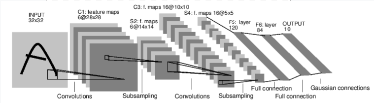
convnet
It is a simple feed-forward network. It takes the input, feeds it through several layers one after the other, and then finally gives the output.
A typical training procedure for a neural network is as follows:
- Define the neural network that has some learnable parameters (or weights)
- Iterate over a dataset of inputs
- Process input through the network
- Compute the loss (how far is the output from being correct)
- Propagate gradients back into the network’s parameters
- Update the weights of the network, typically using a simple update rule:
weight = weight - learning_rate *gradient
Define the network
Let’s define this network:
import torch
import torch.nn as nn
import torch.nn.functional as F


class Net(nn.Module):

    def __init__(self):
        super(Net, self).__init__()
        # 1 input image channel, 6 output channels, 5x5 square convolution
        # kernel
        self.conv1 = nn.Conv2d(1, 6, 5)
        self.conv2 = nn.Conv2d(6, 16, 5)
        # an affine operation: y = Wx + b
        self.fc1 = nn.Linear(16 * 5 * 5, 120)
        self.fc2 = nn.Linear(120, 84)
        self.fc3 = nn.Linear(84, 10)

    def forward(self, x):
        # Max pooling over a (2, 2) window
        x = F.max_pool2d(F.relu(self.conv1(x)), (2, 2))
        # If the size is a square you can only specify a single number
        x = F.max_pool2d(F.relu(self.conv2(x)), 2)
        x = x.view(-1, self.num_flat_features(x))
        x = F.relu(self.fc1(x))
        x = F.relu(self.fc2(x))
        x = self.fc3(x)
        return x

    def num_flat_features(self, x):
        size = x.size()[1:]  # all dimensions except the batch dimension
        num_features = 1
        for s in size:
            num_features *= s
        return num_features


net = Net()
print(net)
Out:
Net(
  (conv1): Conv2d(1, 6, kernel_size=(5, 5), stride=(1, 1))
  (conv2): Conv2d(6, 16, kernel_size=(5, 5), stride=(1, 1))
  (fc1): Linear(in_features=400, out_features=120, bias=True)
  (fc2): Linear(in_features=120, out_features=84, bias=True)
  (fc3): Linear(in_features=84, out_features=10, bias=True)
)
You just have to define the forward function, and the backward function (where gradients are computed) is automatically defined for you using autograd. You can use any of the Tensor operations in the forward function.
The learnable parameters of a model are returned by net.parameters()
params = list(net.parameters())
print(len(params))
print(params[0].size())  # conv1's .weight
Out:
10
torch.Size([6, 1, 5, 5])
Let try a random 32x32 input. Note: expected input size of this net (LeNet) is 32x32. To use this net on MNIST dataset, please resize the images from the dataset to 32x32.
input = torch.randn(1, 1, 32, 32)
out = net(input)
print(out)
Out:
tensor([[-0.0303,  0.0370,  0.1239,  0.0534,  0.0178,  0.0108,  0.0904,  0.1209,
         -0.0256, -0.0081]], grad_fn=<AddmmBackward>)
Zero the gradient buffers of all parameters and backprops with random gradients:
net.zero_grad()
out.backward(torch.randn(1, 10))
NOTE
torch.nn only supports mini-batches. The entire torch.nn package only supports inputs that are a mini-batch of samples, and not a single sample.
For example, nn.Conv2d will take in a 4D Tensor of nSamples x nChannels x Height x Width.
If you have a single sample, just use input.unsqueeze(0) to add a fake batch dimension.
Before proceeding further, let’s recap all the classes you’ve seen so far.
Recap:
torch.Tensor- A multi-dimensional array with support for autograd operations likebackward(). Also holds the gradient w.r.t. the tensor.nn.Module- Neural network module. Convenient way of encapsulating parameters, with helpers for moving them to GPU, exporting, loading, etc.nn.Parameter- A kind of Tensor, that is automatically registered as a parameter when assigned as an attribute to aModule.autograd.Function- Implements forward and backward definitions of an autograd operation. EveryTensoroperation creates at least a singleFunctionnode that connects to functions that created aTensorand encodes its history.
At this point, we covered:
- Defining a neural network
- Processing inputs and calling backward
Still Left:
- Computing the loss
- Updating the weights of the network
Loss Function
A loss function takes the (output, target) pair of inputs, and computes a value that estimates how far away the output is from the target.
There are several different loss functions under the nn package . A simple loss is: nn.MSELoss which computes the mean-squared error between the input and the target.
For example:
output = net(input)
target = torch.randn(10)  # a dummy target, for example
target = target.view(1, -1)  # make it the same shape as output
criterion = nn.MSELoss()

loss = criterion(output, target)
print(loss)
Out:
tensor(1.2616, grad_fn=<MseLossBackward>)
Now, if you follow loss in the backward direction, using its .grad_fn attribute, you will see a graph of computations that looks like this:
input -> conv2d -> relu -> maxpool2d -> conv2d -> relu -> maxpool2d
      -> view -> linear -> relu -> linear -> relu -> linear
      -> MSELoss
      -> loss
So, when we call loss.backward(), the whole graph is differentiated w.r.t. the loss, and all Tensors in the graph that has requires_grad=True will have their .grad Tensor accumulated with the gradient.
For illustration, let us follow a few steps backward:
print(loss.grad_fn)  # MSELoss
print(loss.grad_fn.next_functions[0][0])  # Linear
print(loss.grad_fn.next_functions[0][0].next_functions[0][0])  # ReLU
Out:
<MseLossBackward object at 0x7fb3ce12ae80>
<AddmmBackward object at 0x7fb3ce12a9e8>
<AccumulateGrad object at 0x7fb3ce12a9e8>
Backprop
To backpropagate the error all we have to do is to loss.backward(). You need to clear the existing gradients though, else gradients will be accumulated to existing gradients.
Now we shall call loss.backward(), and have a look at conv1’s bias gradients before and after the backward.
net.zero_grad()     # zeroes the gradient buffers of all parameters

print('conv1.bias.grad before backward')
print(net.conv1.bias.grad)

loss.backward()

print('conv1.bias.grad after backward')
print(net.conv1.bias.grad)
Out:
conv1.bias.grad before backward
tensor([0., 0., 0., 0., 0., 0.])
conv1.bias.grad after backward
tensor([-0.0027,  0.0035,  0.0089, -0.0094,  0.0157,  0.0094])
Now, we have seen how to use loss functions.
Read Later:
The neural network package contains various modules and loss functions that form the building blocks of deep neural networks. A full list with documentation is here.
The only thing left to learn is:
- Updating the weights of the network
Update the weights
The simplest update rule used in practice is the Stochastic Gradient Descent (SGD):
weight = weight - learning_rate * gradient
We can implement this using simple python code:
learning_rate = 0.01
for f in net.parameters():
    f.data.sub_(f.grad.data * learning_rate)
However, as you use neural networks, you want to use various different update rules such as SGD, Nesterov-SGD, Adam, RMSProp, etc. To enable this, we built a small package: torch.optim that implements all these methods. Using it is very simple:
import torch.optim as optim

# create your optimizer
optimizer = optim.SGD(net.parameters(), lr=0.01)

# in your training loop:
optimizer.zero_grad()   # zero the gradient buffers
output = net(input)
loss = criterion(output, target)
loss.backward()
optimizer.step()    # Does the update
NOTE
Observe how gradient buffers had to be manually set to zero using optimizer.zero_grad(). This is because gradients are accumulated as explained in Backprop section.
Total running time of the script: ( 0 minutes 0.106 seconds)
TRAINING A CLASSIFIER
This is it. You have seen how to define neural networks, compute loss and make updates to the weights of the network.
Now you might be thinking,
What about data?
Generally, when you have to deal with image, text, audio or video data, you can use standard python packages that load data into a numpy array. Then you can convert this array into a torch.*Tensor.
- For images, packages such as Pillow, OpenCV are useful
- For audio, packages such as scipy and librosa
- For text, either raw Python or Cython based loading, or NLTK and SpaCy are useful
Specifically for vision, we have created a package called torchvision, that has data loaders for common datasets such as Imagenet, CIFAR10, MNIST, etc. and data transformers for images, viz., torchvision.datasets and torch.utils.data.DataLoader.
This provides a huge convenience and avoids writing boilerplate code.
For this tutorial, we will use the CIFAR10 dataset. It has the classes: ‘airplane’, ‘automobile’, ‘bird’, ‘cat’, ‘deer’, ‘dog’, ‘frog’, ‘horse’, ‘ship’, ‘truck’. The images in CIFAR-10 are of size 3x32x32, i.e. 3-channel color images of 32x32 pixels in size.
cifar10
Training an image classifier
We will do the following steps in order:
- Load and normalizing the CIFAR10 training and test datasets using
torchvision - Define a Convolutional Neural Network
- Define a loss function
- Train the network on the training data
- Test the network on the test data
1. Loading and normalizing CIFAR10
Using torchvision, it’s extremely easy to load CIFAR10.
import torch
import torchvision
import torchvision.transforms as transforms
The output of torchvision datasets are PILImage images of range [0, 1]. We transform them to Tensors of normalized range [-1, 1].
transform = transforms.Compose(
    [transforms.ToTensor(),
     transforms.Normalize((0.5, 0.5, 0.5), (0.5, 0.5, 0.5))])

trainset = torchvision.datasets.CIFAR10(root='./data', train=True,
                                        download=True, transform=transform)
trainloader = torch.utils.data.DataLoader(trainset, batch_size=4,
                                          shuffle=True, num_workers=2)

testset = torchvision.datasets.CIFAR10(root='./data', train=False,
                                       download=True, transform=transform)
testloader = torch.utils.data.DataLoader(testset, batch_size=4,
                                         shuffle=False, num_workers=2)

classes = ('plane', 'car', 'bird', 'cat',
           'deer', 'dog', 'frog', 'horse', 'ship', 'truck')
Out:
Downloading https://www.cs.toronto.edu/~kriz/cifar-10-python.tar.gz to ./data/cifar-10-python.tar.gz
Files already downloaded and verified
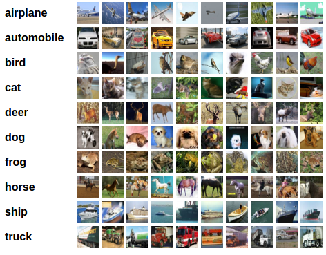
Let us show some of the training images, for fun.
import matplotlib.pyplot as plt
import numpy as np

# functions to show an image


def imshow(img):
    img = img / 2 + 0.5     # unnormalize
    npimg = img.numpy()
    plt.imshow(np.transpose(npimg, (1, 2, 0)))
    plt.show()


# get some random training images
dataiter = iter(trainloader)
images, labels = dataiter.next()

# show images
imshow(torchvision.utils.make_grid(images))
# print labels
print(' '.join('%5s' % classes[labels[j]] for j in range(4)))
Out:
dog frog ship bird
2. Define a Convolutional Neural Network
Copy the neural network from the Neural Networks section before and modify it to take 3-channel images (instead of 1-channel images as it was defined).
import torch.nn as nn
import torch.nn.functional as F


class Net(nn.Module):
    def __init__(self):
        super(Net, self).__init__()
        self.conv1 = nn.Conv2d(3, 6, 5)
        self.pool = nn.MaxPool2d(2, 2)
        self.conv2 = nn.Conv2d(6, 16, 5)
        self.fc1 = nn.Linear(16 * 5 * 5, 120)
        self.fc2 = nn.Linear(120, 84)
        self.fc3 = nn.Linear(84, 10)

    def forward(self, x):
        x = self.pool(F.relu(self.conv1(x)))
        x = self.pool(F.relu(self.conv2(x)))
        x = x.view(-1, 16 * 5 * 5)
        x = F.relu(self.fc1(x))
        x = F.relu(self.fc2(x))
        x = self.fc3(x)
        return x


net = Net()
3. Define a Loss function and optimizer
Let’s use a Classification Cross-Entropy loss and SGD with momentum.
import torch.optim as optim

criterion = nn.CrossEntropyLoss()
optimizer = optim.SGD(net.parameters(), lr=0.001, momentum=0.9)
4. Train the network
This is when things start to get interesting. We simply have to loop over our data iterator, and feed the inputs to the network and optimize.
for epoch in range(2):  # loop over the dataset multiple times

    running_loss = 0.0
    for i, data in enumerate(trainloader, 0):
        # get the inputs
        inputs, labels = data

        # zero the parameter gradients
        optimizer.zero_grad()

        # forward + backward + optimize
        outputs = net(inputs)
        loss = criterion(outputs, labels)
        loss.backward()
        optimizer.step()

        # print statistics
        running_loss += loss.item()
        if i % 2000 == 1999:    # print every 2000 mini-batches
            print('[%d, %5d] loss: %.3f' %
                  (epoch + 1, i + 1, running_loss / 2000))
            running_loss = 0.0

print('Finished Training')
Out:
[1,  2000] loss: 2.132
[1,  4000] loss: 1.793
[1,  6000] loss: 1.656
[1,  8000] loss: 1.599
[1, 10000] loss: 1.545
[1, 12000] loss: 1.501
[2,  2000] loss: 1.432
[2,  4000] loss: 1.406
[2,  6000] loss: 1.386
[2,  8000] loss: 1.373
[2, 10000] loss: 1.351
[2, 12000] loss: 1.300
Finished Training
5. Test the network on the test data
We have trained the network for 2 passes over the training dataset. But we need to check if the network has learnt anything at all.
We will check this by predicting the class label that the neural network outputs, and checking it against the ground-truth. If the prediction is correct, we add the sample to the list of correct predictions.
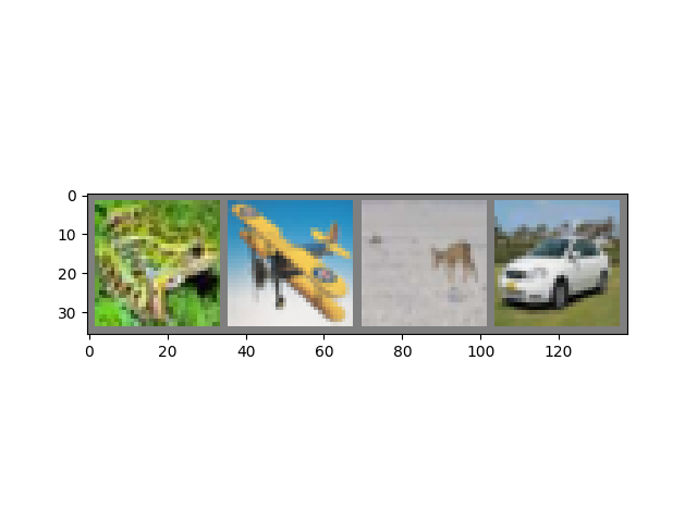
Okay, first step. Let us display an image from the test set to get familiar.
dataiter = iter(testloader)
images, labels = dataiter.next()

# print images
imshow(torchvision.utils.make_grid(images))
print('GroundTruth: ', ' '.join('%5s' % classes[labels[j]] for j in range(4)))
Out:
GroundTruth: cat ship ship plane
Okay, now let us see what the neural network thinks these examples above are:
outputs = net(images)
The outputs are energies for the 10 classes. The higher the energy for a class, the more the network thinks that the image is of the particular class. So, let’s get the index of the highest energy:
_, predicted = torch.max(outputs, 1)

print('Predicted: ', ' '.join('%5s' % classes[predicted[j]]
                              for j in range(4)))
Out:
Predicted: cat car car plane
The results seem pretty good.
Let us look at how the network performs on the whole dataset.
correct = 0
total = 0
with torch.no_grad():
    for data in testloader:
        images, labels = data
        outputs = net(images)
        _, predicted = torch.max(outputs.data, 1)
        total += labels.size(0)
        correct += (predicted == labels).sum().item()

print('Accuracy of the network on the 10000 test images: %d %%' % (
    100 * correct / total))
Out:
Accuracy of the network on the 10000 test images: 52 %
That looks waaay better than chance, which is 10% accuracy (randomly picking a class out of 10 classes). Seems like the network learnt something.
Hmmm, what are the classes that performed well, and the classes that did not perform well:
class_correct = list(0. for i in range(10))
class_total = list(0. for i in range(10))
with torch.no_grad():
    for data in testloader:
        images, labels = data
        outputs = net(images)
        _, predicted = torch.max(outputs, 1)
        c = (predicted == labels).squeeze()
        for i in range(4):
            label = labels[i]
            class_correct[label] += c[i].item()
            class_total[label] += 1


for i in range(10):
    print('Accuracy of %5s : %2d %%' % (
        classes[i], 100 * class_correct[i] / class_total[i]))
Out:
Accuracy of plane : 62 %
Accuracy of   car : 51 %
Accuracy of  bird : 53 %
Accuracy of   cat : 25 %
Accuracy of  deer : 26 %
Accuracy of   dog : 56 %
Accuracy of  frog : 66 %
Accuracy of horse : 67 %
Accuracy of  ship : 44 %
Accuracy of truck : 74 %
Okay, so what next?
How do we run these neural networks on the GPU?
Training on GPU
Just like how you transfer a Tensor onto the GPU, you transfer the neural net onto the GPU.
Let’s first define our device as the first visible cuda device if we have CUDA available:
device = torch.device("cuda:0" if torch.cuda.is_available() else "cpu")

# Assuming that we are on a CUDA machine, this should print a CUDA device:

print(device)
Out:
cuda:0
The rest of this section assumes that device is a CUDA device.
Then these methods will recursively go over all modules and convert their parameters and buffers to CUDA tensors:
net.to(device)
Remember that you will have to send the inputs and targets at every step to the GPU too:
inputs, labels = inputs.to(device), labels.to(device)
Why dont I notice MASSIVE speedup compared to CPU? Because your network is realllly small.
Exercise: Try increasing the width of your network (argument 2 of the first nn.Conv2d, and argument 1 of the second nn.Conv2d – they need to be the same number), see what kind of speedup you get.
Goals achieved:
- Understanding PyTorch’s Tensor library and neural networks at a high level.
- Train a small neural network to classify images
Training on multiple GPUs
If you want to see even more MASSIVE speedup using all of your GPUs, please check out Optional: Data Parallelism.
Where do I go next?
- Train neural nets to play video games
- Train a state-of-the-art ResNet network on imagenet
- Train a face generator using Generative Adversarial Networks
- Train a word-level language model using Recurrent LSTM networks
- More examples
- More tutorials
- Discuss PyTorch on the Forums
- Chat with other users on Slack
# %%%%%%INVISIBLE_CODE_BLOCK%%%%%%
del dataiter
# %%%%%%INVISIBLE_CODE_BLOCK%%%%%%
Total running time of the script: ( 4 minutes 43.859 seconds)
OPTIONAL: DATA PARALLELISM
Authors: Sung Kim and Jenny Kang
In this tutorial, we will learn how to use multiple GPUs using DataParallel.
It’s very easy to use GPUs with PyTorch. You can put the model on a GPU:
device = torch.device("cuda:0")
model.to(device)
Then, you can copy all your tensors to the GPU:
mytensor = my_tensor.to(device)
Please note that just calling my_tensor.to(device) returns a new copy of my_tensor on GPU instead of rewriting my_tensor. You need to assign it to a new tensor and use that tensor on the GPU.
It’s natural to execute your forward, backward propagations on multiple GPUs. However, Pytorch will only use one GPU by default. You can easily run your operations on multiple GPUs by making your model run parallelly using DataParallel:
model = nn.DataParallel(model)
That’s the core behind this tutorial. We will explore it in more detail below.
Imports and parameters
Import PyTorch modules and define parameters.
import torch
import torch.nn as nn
from torch.utils.data import Dataset, DataLoader

# Parameters and DataLoaders
input_size = 5
output_size = 2

batch_size = 30
data_size = 100
Device
device = torch.device("cuda:0" if torch.cuda.is_available() else "cpu")
Dummy DataSet
Make a dummy (random) dataset. You just need to implement the getitem
class RandomDataset(Dataset):

    def __init__(self, size, length):
        self.len = length
        self.data = torch.randn(length, size)

    def __getitem__(self, index):
        return self.data[index]

    def __len__(self):
        return self.len

rand_loader = DataLoader(dataset=RandomDataset(input_size, data_size),
                         batch_size=batch_size, shuffle=True)
Simple Model
For the demo, our model just gets an input, performs a linear operation, and gives an output. However, you can use DataParallel on any model (CNN, RNN, Capsule Net etc.)
We’ve placed a print statement inside the model to monitor the size of input and output tensors. Please pay attention to what is printed at batch rank 0.
class Model(nn.Module):
    # Our model

    def __init__(self, input_size, output_size):
        super(Model, self).__init__()
        self.fc = nn.Linear(input_size, output_size)

    def forward(self, input):
        output = self.fc(input)
        print("\tIn Model: input size", input.size(),
              "output size", output.size())

        return output
Create Model and DataParallel
This is the core part of the tutorial. First, we need to make a model instance and check if we have multiple GPUs. If we have multiple GPUs, we can wrap our model using nn.DataParallel. Then we can put our model on GPUs by model.to(device)
model = Model(input_size, output_size)
if torch.cuda.device_count() > 1:
  print("Let's use", torch.cuda.device_count(), "GPUs!")
  # dim = 0 [30, xxx] -> [10, ...], [10, ...], [10, ...] on 3 GPUs
  model = nn.DataParallel(model)

model.to(device)
Out:
Let's use 2 GPUs!
Run the Model
Now we can see the sizes of input and output tensors.
for data in rand_loader:
    input = data.to(device)
    output = model(input)
    print("Outside: input size", input.size(),
          "output_size", output.size())
Out:
In Model: input size    In Model: input size torch.Size([15, 5]) output size torch.Size([15, 2])
 torch.Size([15, 5]) output size torch.Size([15, 2])
Outside: input size torch.Size([30, 5]) output_size torch.Size([30, 2])
        In Model: input size torch.Size([15, 5]) output size torch.Size([15, 2])
        In Model: input size torch.Size([15, 5]) output size torch.Size([15, 2])
Outside: input size torch.Size([30, 5]) output_size torch.Size([30, 2])
        In Model: input size torch.Size([15, 5]) output size torch.Size([15, 2])
        In Model: input size torch.Size([15, 5]) output size torch.Size([15, 2])
Outside: input size torch.Size([30, 5]) output_size torch.Size([30, 2])
        In Model: input size torch.Size([5, 5]) output size torch.Size([5, 2])
        In Model: input size torch.Size([5, 5]) output size torch.Size([5, 2])
Outside: input size torch.Size([10, 5]) output_size torch.Size([10, 2])
Results
If you have no GPU or one GPU, when we batch 30 inputs and 30 outputs, the model gets 30 and outputs 30 as expected. But if you have multiple GPUs, then you can get results like this.
2 GPUs
If you have 2, you will see:
# on 2 GPUs
Let's use 2 GPUs!
    In Model: input size torch.Size([15, 5]) output size torch.Size([15, 2])
    In Model: input size torch.Size([15, 5]) output size torch.Size([15, 2])
Outside: input size torch.Size([30, 5]) output_size torch.Size([30, 2])
    In Model: input size torch.Size([15, 5]) output size torch.Size([15, 2])
    In Model: input size torch.Size([15, 5]) output size torch.Size([15, 2])
Outside: input size torch.Size([30, 5]) output_size torch.Size([30, 2])
    In Model: input size torch.Size([15, 5]) output size torch.Size([15, 2])
    In Model: input size torch.Size([15, 5]) output size torch.Size([15, 2])
Outside: input size torch.Size([30, 5]) output_size torch.Size([30, 2])
    In Model: input size torch.Size([5, 5]) output size torch.Size([5, 2])
    In Model: input size torch.Size([5, 5]) output size torch.Size([5, 2])
Outside: input size torch.Size([10, 5]) output_size torch.Size([10, 2])
3 GPUs
If you have 3 GPUs, you will see:
Let's use 3 GPUs!
    In Model: input size torch.Size([10, 5]) output size torch.Size([10, 2])
    In Model: input size torch.Size([10, 5]) output size torch.Size([10, 2])
    In Model: input size torch.Size([10, 5]) output size torch.Size([10, 2])
Outside: input size torch.Size([30, 5]) output_size torch.Size([30, 2])
    In Model: input size torch.Size([10, 5]) output size torch.Size([10, 2])
    In Model: input size torch.Size([10, 5]) output size torch.Size([10, 2])
    In Model: input size torch.Size([10, 5]) output size torch.Size([10, 2])
Outside: input size torch.Size([30, 5]) output_size torch.Size([30, 2])
    In Model: input size torch.Size([4, 5]) output size torch.Size([4, 2])
    In Model: input size torch.Size([4, 5]) output size torch.Size([4, 2])
    In Model: input size torch.Size([2, 5]) output size torch.Size([2, 2])
Outside: input size torch.Size([10, 5]) output_size torch.Size([10, 2])
8 GPUs
If you have 8, you will see:
Let's use 8 GPUs!
    In Model: input size torch.Size([4, 5]) output size torch.Size([4, 2])
    In Model: input size torch.Size([4, 5]) output size torch.Size([4, 2])
    In Model: input size torch.Size([2, 5]) output size torch.Size([2, 2])
    In Model: input size torch.Size([4, 5]) output size torch.Size([4, 2])
    In Model: input size torch.Size([4, 5]) output size torch.Size([4, 2])
    In Model: input size torch.Size([4, 5]) output size torch.Size([4, 2])
    In Model: input size torch.Size([4, 5]) output size torch.Size([4, 2])
    In Model: input size torch.Size([4, 5]) output size torch.Size([4, 2])
Outside: input size torch.Size([30, 5]) output_size torch.Size([30, 2])
    In Model: input size torch.Size([4, 5]) output size torch.Size([4, 2])
    In Model: input size torch.Size([4, 5]) output size torch.Size([4, 2])
    In Model: input size torch.Size([4, 5]) output size torch.Size([4, 2])
    In Model: input size torch.Size([4, 5]) output size torch.Size([4, 2])
    In Model: input size torch.Size([4, 5]) output size torch.Size([4, 2])
    In Model: input size torch.Size([4, 5]) output size torch.Size([4, 2])
    In Model: input size torch.Size([2, 5]) output size torch.Size([2, 2])
    In Model: input size torch.Size([4, 5]) output size torch.Size([4, 2])
Outside: input size torch.Size([30, 5]) output_size torch.Size([30, 2])
    In Model: input size torch.Size([4, 5]) output size torch.Size([4, 2])
    In Model: input size torch.Size([4, 5]) output size torch.Size([4, 2])
    In Model: input size torch.Size([4, 5]) output size torch.Size([4, 2])
    In Model: input size torch.Size([4, 5]) output size torch.Size([4, 2])
    In Model: input size torch.Size([4, 5]) output size torch.Size([4, 2])
    In Model: input size torch.Size([4, 5]) output size torch.Size([4, 2])
    In Model: input size torch.Size([4, 5]) output size torch.Size([4, 2])
    In Model: input size torch.Size([2, 5]) output size torch.Size([2, 2])
Outside: input size torch.Size([30, 5]) output_size torch.Size([30, 2])
    In Model: input size torch.Size([2, 5]) output size torch.Size([2, 2])
    In Model: input size torch.Size([2, 5]) output size torch.Size([2, 2])
    In Model: input size torch.Size([2, 5]) output size torch.Size([2, 2])
    In Model: input size torch.Size([2, 5]) output size torch.Size([2, 2])
    In Model: input size torch.Size([2, 5]) output size torch.Size([2, 2])
Outside: input size torch.Size([10, 5]) output_size torch.Size([10, 2])
Summary
DataParallel splits your data automatically and sends job orders to multiple models on several GPUs. After each model finishes their job, DataParallel collects and merges the results before returning it to you.
For more information, please check out https://pytorch.org/tutorials/beginner/former_torchies/parallelism_tutorial.html.
Total running time of the script: ( 0 minutes 8.918 seconds)