版权声明:本文为博主原创文章,未经博主允许不得转载。 https://blog.csdn.net/xd15010130025/article/details/88723032
我们来复习上一节的知识:
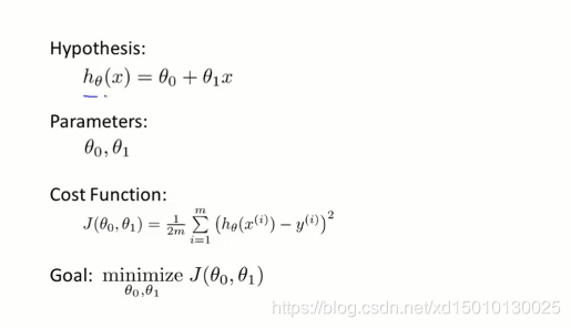
假设函数:
hθ(x)=θ0+θ1x
参数:
θ0,θ1
代价函数:
J(θ0,θ1)=2m1∑i=1i=m(h(xi)−yi)2
目标:求得当
J(θ0,θ1)最小时的
θ0,θ1值
做一个简化,令:
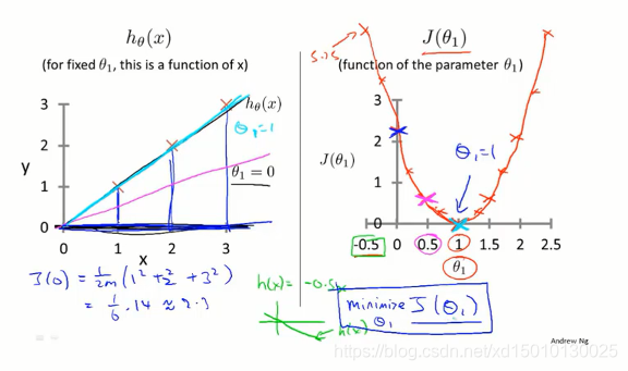
hθ(x)=θ1x
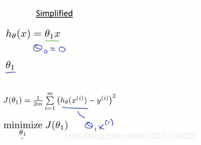
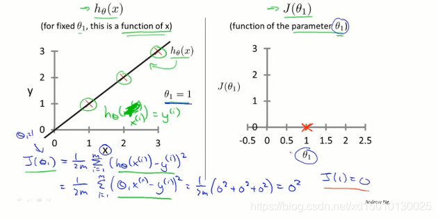
我们可以画出假设函数和代价函数的值。可知,当
θ1=1时,有
hθ(x)=x
J(θ1=1)=2∗31∗[(1−1)2+(2−2)2+(3−3)2]=0
当
θ1=0.5时,有
hθ(x)=0.5x
J(θ1=0.5)=2∗31∗[(0.5−1)2+(1−2)2+(1.5−3)2]=0.58
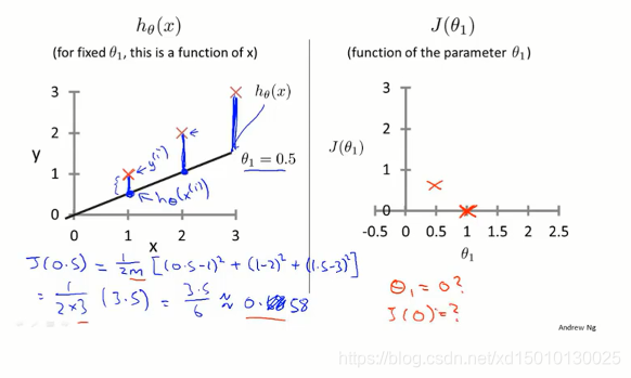
当
θ1=0时,有
hθ(x)=0
J(θ1=0)=2∗31∗[(0−1)2+(0−2)2+(0−3)2]=2.3
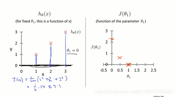
据此我们可以作出
hθ(x)和
J(θ1)的图
下次我们将继续讨论加上
θ0的情形