版权声明:此文章有作者原创,涉及相关版本问题可以联系作者,[email protected] https://blog.csdn.net/weixin_42600072/article/details/88644810
beer数据集 聚类分析
import pandas as pd

beer = pd.read_csv('./data/data.txt', sep=' ')
print(beer)
                    name  calories  sodium  alcohol  cost
0              Budweiser       144      15      4.7  0.43
1                Schlitz       151      19      4.9  0.43
2              Lowenbrau       157      15      0.9  0.48
3            Kronenbourg       170       7      5.2  0.73
4               Heineken       152      11      5.0  0.77
5          Old_Milwaukee       145      23      4.6  0.28
6             Augsberger       175      24      5.5  0.40
7   Srohs_Bohemian_Style       149      27      4.7  0.42
8            Miller_Lite        99      10      4.3  0.43
9        Budweiser_Light       113       8      3.7  0.40
10                 Coors       140      18      4.6  0.44
11           Coors_Light       102      15      4.1  0.46
12        Michelob_Light       135      11      4.2  0.50
13                 Becks       150      19      4.7  0.76
14                 Kirin       149       6      5.0  0.79
15     Pabst_Extra_Light        68      15      2.3  0.38
16                 Hamms       139      19      4.4  0.43
17   Heilemans_Old_Style       144      24      4.9  0.43
18   Olympia_Goled_Light        72       6      2.9  0.46
19         Schlitz_Light        97       7      4.2  0.47
X = beer[['calories', 'sodium', 'alcohol', 'cost']]
K-means聚类算法
from sklearn.cluster import KMeans

km = KMeans(n_clusters=3).fit(X)
km2 = KMeans(n_clusters=2).fit(X)
km.labels_
array([0, 0, 0, 0, 0, 0, 0, 0, 2, 2, 0, 2, 0, 0, 0, 1, 0, 0, 1, 2])
beer['cluster'] = km.labels_
beer['cluster2'] = km2.labels_
beer.sort_values('cluster')
| name | calories | sodium | alcohol | cost | cluster | cluster2 | |
|---|---|---|---|---|---|---|---|
| 0 | Budweiser | 144 | 15 | 4.7 | 0.43 | 0 | 0 |
| 1 | Schlitz | 151 | 19 | 4.9 | 0.43 | 0 | 0 |
| 2 | Lowenbrau | 157 | 15 | 0.9 | 0.48 | 0 | 0 |
| 3 | Kronenbourg | 170 | 7 | 5.2 | 0.73 | 0 | 0 |
| 4 | Heineken | 152 | 11 | 5.0 | 0.77 | 0 | 0 |
| 5 | Old_Milwaukee | 145 | 23 | 4.6 | 0.28 | 0 | 0 |
| 6 | Augsberger | 175 | 24 | 5.5 | 0.40 | 0 | 0 |
| 7 | Srohs_Bohemian_Style | 149 | 27 | 4.7 | 0.42 | 0 | 0 |
| 17 | Heilemans_Old_Style | 144 | 24 | 4.9 | 0.43 | 0 | 0 |
| 10 | Coors | 140 | 18 | 4.6 | 0.44 | 0 | 0 |
| 16 | Hamms | 139 | 19 | 4.4 | 0.43 | 0 | 0 |
| 12 | Michelob_Light | 135 | 11 | 4.2 | 0.50 | 0 | 0 |
| 13 | Becks | 150 | 19 | 4.7 | 0.76 | 0 | 0 |
| 14 | Kirin | 149 | 6 | 5.0 | 0.79 | 0 | 0 |
| 18 | Olympia_Goled_Light | 72 | 6 | 2.9 | 0.46 | 1 | 1 |
| 15 | Pabst_Extra_Light | 68 | 15 | 2.3 | 0.38 | 1 | 1 |
| 9 | Budweiser_Light | 113 | 8 | 3.7 | 0.40 | 2 | 1 |
| 8 | Miller_Lite | 99 | 10 | 4.3 | 0.43 | 2 | 1 |
| 11 | Coors_Light | 102 | 15 | 4.1 | 0.46 | 2 | 1 |
| 19 | Schlitz_Light | 97 | 7 | 4.2 | 0.47 | 2 | 1 |
from pandas.tools.plotting import scatter_matrix
%matplotlib inline

cluster_centers = km.cluster_centers_
cluster2_centers = km2.cluster_centers_
beer.groupby('cluster').mean()
| calories | sodium | alcohol | cost | cluster2 | |
|---|---|---|---|---|---|
| cluster | |||||
| 0 | 150.00 | 17.0 | 4.521429 | 0.520714 | 0 |
| 1 | 70.00 | 10.5 | 2.600000 | 0.420000 | 1 |
| 2 | 102.75 | 10.0 | 4.075000 | 0.440000 | 1 |
beer.groupby('cluster2').mean()
| calories | sodium | alcohol | cost | cluster | |
|---|---|---|---|---|---|
| cluster2 | |||||
| 0 | 150.000000 | 17.000000 | 4.521429 | 0.520714 | 0.000000 |
| 1 | 91.833333 | 10.166667 | 3.583333 | 0.433333 | 1.666667 |
centers = beer.groupby('cluster').mean().reset_index()
import matplotlib.pyplot as plt

plt.rcParams['font.size'] = 14
import numpy as np

colors = np.array(['red', 'green', 'blue', 'yellow'])
plt.scatter(beer['calories'], beer['alcohol'], c = colors[beer['cluster']])
plt.scatter(centers.calories, centers.alcohol, linewidths=3, marker='+', s=300, c='black')

plt.xlabel('calories')
plt.ylabel('alcohol')
Text(0, 0.5, 'alcohol')

scatter_matrix(beer[["calories","sodium","alcohol","cost"]],s=100, alpha=1, c=colors[beer["cluster"]], figsize=(10,10))
plt.suptitle("With 3 centroids initialized")
C:\ProgramData\Anaconda3\lib\site-packages\ipykernel_launcher.py:1: FutureWarning: 'pandas.tools.plotting.scatter_matrix' is deprecated, import 'pandas.plotting.scatter_matrix' instead.
  """Entry point for launching an IPython kernel.


Text(0.5, 0.98, 'With 3 centroids initialized')

scatter_matrix(beer[['calories','sodium','alcohol','cost']],s=100, alpha=1, c=colors[beer['cluster2']], figsize=(10,10))
plt.suptitle('With 2 centroids initialized')
C:\ProgramData\Anaconda3\lib\site-packages\ipykernel_launcher.py:1: FutureWarning: 'pandas.tools.plotting.scatter_matrix' is deprecated, import 'pandas.plotting.scatter_matrix' instead.
  """Entry point for launching an IPython kernel.


Text(0.5, 0.98, 'With 2 centroids initialized')

数据标准化或归一化
from sklearn.preprocessing import StandardScaler

scaler = StandardScaler()
X_scaled = scaler.fit_transform(X)
X_scaled
C:\ProgramData\Anaconda3\lib\site-packages\sklearn\preprocessing\data.py:625: DataConversionWarning: Data with input dtype int64, float64 were all converted to float64 by StandardScaler.
  return self.partial_fit(X, y)
C:\ProgramData\Anaconda3\lib\site-packages\sklearn\base.py:462: DataConversionWarning: Data with input dtype int64, float64 were all converted to float64 by StandardScaler.
  return self.fit(X, **fit_params).transform(X)


array([[ 0.38791334,  0.00779468,  0.43380786, -0.45682969],
       [ 0.6250656 ,  0.63136906,  0.62241997, -0.45682969],
       [ 0.82833896,  0.00779468, -3.14982226, -0.10269815],
       [ 1.26876459, -1.23935408,  0.90533814,  1.66795955],
       [ 0.65894449, -0.6157797 ,  0.71672602,  1.95126478],
       [ 0.42179223,  1.25494344,  0.3395018 , -1.5192243 ],
       [ 1.43815906,  1.41083704,  1.1882563 , -0.66930861],
       [ 0.55730781,  1.87851782,  0.43380786, -0.52765599],
       [-1.1366369 , -0.7716733 ,  0.05658363, -0.45682969],
       [-0.66233238, -1.08346049, -0.5092527 , -0.66930861],
       [ 0.25239776,  0.47547547,  0.3395018 , -0.38600338],
       [-1.03500022,  0.00779468, -0.13202848, -0.24435076],
       [ 0.08300329, -0.6157797 , -0.03772242,  0.03895447],
       [ 0.59118671,  0.63136906,  0.43380786,  1.88043848],
       [ 0.55730781, -1.39524768,  0.71672602,  2.0929174 ],
       [-2.18688263,  0.00779468, -1.82953748, -0.81096123],
       [ 0.21851887,  0.63136906,  0.15088969, -0.45682969],
       [ 0.38791334,  1.41083704,  0.62241997, -0.45682969],
       [-2.05136705, -1.39524768, -1.26370115, -0.24435076],
       [-1.20439469, -1.23935408, -0.03772242, -0.17352445]])
km = KMeans(n_clusters=3).fit(X_scaled)
beer['scaled_cluster'] = km.labels_
beer.sort_values('scaled_cluster')
| name | calories | sodium | alcohol | cost | cluster | cluster2 | scaled_cluster | |
|---|---|---|---|---|---|---|---|---|
| 0 | Budweiser | 144 | 15 | 4.7 | 0.43 | 0 | 0 | 0 |
| 1 | Schlitz | 151 | 19 | 4.9 | 0.43 | 0 | 0 | 0 |
| 17 | Heilemans_Old_Style | 144 | 24 | 4.9 | 0.43 | 0 | 0 | 0 |
| 16 | Hamms | 139 | 19 | 4.4 | 0.43 | 0 | 0 | 0 |
| 5 | Old_Milwaukee | 145 | 23 | 4.6 | 0.28 | 0 | 0 | 0 |
| 6 | Augsberger | 175 | 24 | 5.5 | 0.40 | 0 | 0 | 0 |
| 7 | Srohs_Bohemian_Style | 149 | 27 | 4.7 | 0.42 | 0 | 0 | 0 |
| 10 | Coors | 140 | 18 | 4.6 | 0.44 | 0 | 0 | 0 |
| 15 | Pabst_Extra_Light | 68 | 15 | 2.3 | 0.38 | 1 | 1 | 1 |
| 12 | Michelob_Light | 135 | 11 | 4.2 | 0.50 | 0 | 0 | 1 |
| 11 | Coors_Light | 102 | 15 | 4.1 | 0.46 | 2 | 1 | 1 |
| 9 | Budweiser_Light | 113 | 8 | 3.7 | 0.40 | 2 | 1 | 1 |
| 8 | Miller_Lite | 99 | 10 | 4.3 | 0.43 | 2 | 1 | 1 |
| 2 | Lowenbrau | 157 | 15 | 0.9 | 0.48 | 0 | 0 | 1 |
| 18 | Olympia_Goled_Light | 72 | 6 | 2.9 | 0.46 | 1 | 1 | 1 |
| 19 | Schlitz_Light | 97 | 7 | 4.2 | 0.47 | 2 | 1 | 1 |
| 13 | Becks | 150 | 19 | 4.7 | 0.76 | 0 | 0 | 2 |
| 14 | Kirin | 149 | 6 | 5.0 | 0.79 | 0 | 0 | 2 |
| 4 | Heineken | 152 | 11 | 5.0 | 0.77 | 0 | 0 | 2 |
| 3 | Kronenbourg | 170 | 7 | 5.2 | 0.73 | 0 | 0 | 2 |
beer.groupby('scaled_cluster').mean()
| calories | sodium | alcohol | cost | cluster | cluster2 | |
|---|---|---|---|---|---|---|
| scaled_cluster | ||||||
| 0 | 148.375 | 21.125 | 4.7875 | 0.4075 | 0.00 | 0.00 |
| 1 | 105.375 | 10.875 | 3.3250 | 0.4475 | 1.25 | 0.75 |
| 2 | 155.250 | 10.750 | 4.9750 | 0.7625 | 0.00 | 0.00 |
pd.scatter_matrix(X, c=colors[beer.scaled_cluster], alpha=1, figsize=(10,10), s=100)
C:\ProgramData\Anaconda3\lib\site-packages\ipykernel_launcher.py:1: FutureWarning: pandas.scatter_matrix is deprecated, use pandas.plotting.scatter_matrix instead
  """Entry point for launching an IPython kernel.


array([[<matplotlib.axes._subplots.AxesSubplot object at 0x0000000010717630>,
        <matplotlib.axes._subplots.AxesSubplot object at 0x00000000102F2668>,
        <matplotlib.axes._subplots.AxesSubplot object at 0x000000000FFDE8D0>,
        <matplotlib.axes._subplots.AxesSubplot object at 0x000000000FFCFD68>],
       [<matplotlib.axes._subplots.AxesSubplot object at 0x000000001072F208>,
        <matplotlib.axes._subplots.AxesSubplot object at 0x0000000010729470>,
        <matplotlib.axes._subplots.AxesSubplot object at 0x00000000105FA6D8>,
        <matplotlib.axes._subplots.AxesSubplot object at 0x0000000010690DD8>],
       [<matplotlib.axes._subplots.AxesSubplot object at 0x0000000010690E10>,
        <matplotlib.axes._subplots.AxesSubplot object at 0x00000000106242B0>,
        <matplotlib.axes._subplots.AxesSubplot object at 0x0000000010330518>,
        <matplotlib.axes._subplots.AxesSubplot object at 0x000000001033B780>],
       [<matplotlib.axes._subplots.AxesSubplot object at 0x00000000105A89E8>,
        <matplotlib.axes._subplots.AxesSubplot object at 0x00000000102A0C50>,
        <matplotlib.axes._subplots.AxesSubplot object at 0x00000000102BEEB8>,
        <matplotlib.axes._subplots.AxesSubplot object at 0x0000000010574160>]],
      dtype=object)

聚类评估:轮廓系数(Silhouette Coefficient )
 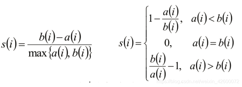 - 计算样本i到同簇其他样本的平均距离ai。ai 越小,说明样本i越应该被聚类到该簇。将ai 称为样本i的簇内不相似度。 - 计算样本i到其他某簇Cj 的所有样本的平均距离bij,称为样本i与簇Cj 的不相似度。定义为样本i的簇间不相似度:bi =min{bi1, bi2, ..., bik}
 - 计算样本i到同簇其他样本的平均距离ai。ai 越小,说明样本i越应该被聚类到该簇。将ai 称为样本i的簇内不相似度。 - 计算样本i到其他某簇Cj 的所有样本的平均距离bij,称为样本i与簇Cj 的不相似度。定义为样本i的簇间不相似度:bi =min{bi1, bi2, ..., bik}
- si接近1,则说明样本i聚类合理
- si接近-1,则说明样本i更应该分类到另外的簇
- 若si 近似为0,则说明样本i在两个簇的边界上。
from sklearn import metrics

score = metrics.silhouette_score(X,beer.cluster)
score_scaled = metrics.silhouette_score(X, beer.scaled_cluster)
print(score, score_scaled)
0.6731775046455796 0.1797806808940007
scores = []
for k in range(2,20):
    labels = KMeans(n_clusters=k).fit(X).labels_
    score = metrics.silhouette_score(X, labels)
    scores.append(score)

scores
[0.6917656034079486,
 0.6731775046455796,
 0.5857040721127795,
 0.4225487335172022,
 0.4559182167013378,
 0.43776116697963136,
 0.38946337473126,
 0.39746405172426014,
 0.3915697409245163,
 0.3413109618039333,
 0.3459775237127248,
 0.31221439248428434,
 0.30707782144770296,
 0.31834561839139497,
 0.2849514001174898,
 0.23498077333071996,
 0.1588091017496281,
 0.08423051380151177]
plt.plot(list(range(2,20)), scores)
plt.xlabel("Number of Clusters Initialized")
plt.ylabel("Sihouette Score")
Text(0, 0.5, 'Sihouette Score')

DBSCAN聚类
from sklearn.cluster import DBSCAN

db = DBSCAN(eps=10, min_samples=2).fit(X)  #半径为10,密度为2
labels = db.labels_
beer['cluster_db'] = labels
beer.sort_values('cluster_db')
| name | calories | sodium | alcohol | cost | cluster | cluster2 | scaled_cluster | cluster_db | |
|---|---|---|---|---|---|---|---|---|---|
| 9 | Budweiser_Light | 113 | 8 | 3.7 | 0.40 | 2 | 1 | 1 | -1 |
| 3 | Kronenbourg | 170 | 7 | 5.2 | 0.73 | 0 | 0 | 2 | -1 |
| 6 | Augsberger | 175 | 24 | 5.5 | 0.40 | 0 | 0 | 0 | -1 |
| 17 | Heilemans_Old_Style | 144 | 24 | 4.9 | 0.43 | 0 | 0 | 0 | 0 |
| 16 | Hamms | 139 | 19 | 4.4 | 0.43 | 0 | 0 | 0 | 0 |
| 14 | Kirin | 149 | 6 | 5.0 | 0.79 | 0 | 0 | 2 | 0 |
| 13 | Becks | 150 | 19 | 4.7 | 0.76 | 0 | 0 | 2 | 0 |
| 12 | Michelob_Light | 135 | 11 | 4.2 | 0.50 | 0 | 0 | 1 | 0 |
| 10 | Coors | 140 | 18 | 4.6 | 0.44 | 0 | 0 | 0 | 0 |
| 0 | Budweiser | 144 | 15 | 4.7 | 0.43 | 0 | 0 | 0 | 0 |
| 7 | Srohs_Bohemian_Style | 149 | 27 | 4.7 | 0.42 | 0 | 0 | 0 | 0 |
| 5 | Old_Milwaukee | 145 | 23 | 4.6 | 0.28 | 0 | 0 | 0 | 0 |
| 4 | Heineken | 152 | 11 | 5.0 | 0.77 | 0 | 0 | 2 | 0 |
| 2 | Lowenbrau | 157 | 15 | 0.9 | 0.48 | 0 | 0 | 1 | 0 |
| 1 | Schlitz | 151 | 19 | 4.9 | 0.43 | 0 | 0 | 0 | 0 |
| 8 | Miller_Lite | 99 | 10 | 4.3 | 0.43 | 2 | 1 | 1 | 1 |
| 11 | Coors_Light | 102 | 15 | 4.1 | 0.46 | 2 | 1 | 1 | 1 |
| 19 | Schlitz_Light | 97 | 7 | 4.2 | 0.47 | 2 | 1 | 1 | 1 |
| 15 | Pabst_Extra_Light | 68 | 15 | 2.3 | 0.38 | 1 | 1 | 1 | 2 |
| 18 | Olympia_Goled_Light | 72 | 6 | 2.9 | 0.46 | 1 | 1 | 1 | 2 |
beer.groupby('cluster_db').mean()
| calories | sodium | alcohol | cost | cluster | cluster2 | scaled_cluster | |
|---|---|---|---|---|---|---|---|
| cluster_db | |||||||
| -1 | 152.666667 | 13.000000 | 4.800000 | 0.510000 | 0.666667 | 0.333333 | 1.000000 |
| 0 | 146.250000 | 17.250000 | 4.383333 | 0.513333 | 0.000000 | 0.000000 | 0.666667 |
| 1 | 99.333333 | 10.666667 | 4.200000 | 0.453333 | 2.000000 | 1.000000 | 1.000000 |
| 2 | 70.000000 | 10.500000 | 2.600000 | 0.420000 | 1.000000 | 1.000000 | 1.000000 |
pd.scatter_matrix(X, c=colors[beer.cluster_db], figsize=(10,10), s=100)
C:\ProgramData\Anaconda3\lib\site-packages\ipykernel_launcher.py:1: FutureWarning: pandas.scatter_matrix is deprecated, use pandas.plotting.scatter_matrix instead
  """Entry point for launching an IPython kernel.


array([[<matplotlib.axes._subplots.AxesSubplot object at 0x00000000107B6F98>,
        <matplotlib.axes._subplots.AxesSubplot object at 0x0000000010542C18>,
        <matplotlib.axes._subplots.AxesSubplot object at 0x000000001042E278>,
        <matplotlib.axes._subplots.AxesSubplot object at 0x00000000107C0208>],
       [<matplotlib.axes._subplots.AxesSubplot object at 0x00000000109376D8>,
        <matplotlib.axes._subplots.AxesSubplot object at 0x0000000010984940>,
        <matplotlib.axes._subplots.AxesSubplot object at 0x0000000012022BA8>,
        <matplotlib.axes._subplots.AxesSubplot object at 0x000000001206C438>],
       [<matplotlib.axes._subplots.AxesSubplot object at 0x000000001206C470>,
        <matplotlib.axes._subplots.AxesSubplot object at 0x0000000011F848D0>,
        <matplotlib.axes._subplots.AxesSubplot object at 0x0000000011F04B38>,
        <matplotlib.axes._subplots.AxesSubplot object at 0x0000000012093DA0>],
       [<matplotlib.axes._subplots.AxesSubplot object at 0x00000000121A6048>,
        <matplotlib.axes._subplots.AxesSubplot object at 0x0000000011F672B0>,
        <matplotlib.axes._subplots.AxesSubplot object at 0x00000000120E5518>,
        <matplotlib.axes._subplots.AxesSubplot object at 0x00000000107AA780>]],
      dtype=object)
