最近一直被训练过程中的Memory Error困扰,查了资料如何避免发生MemoryError,文章解释了python的dictionary分配内存的机制带来的巨大问题,并给出了优化的思路。但是并没有代码示例。
显然理论上明白该怎么做并不能很快速的指引我解决眼下的问题,只是让我明白了方法,具体的操作还在构思,于是继续查资料。无意中发现了这个out-of-core分类器,该思路符合文章里的小批量解决思路。
英文好的可以直接看原文,我的英文阅读水平也就是自己能意会,无法言传的程度。out-of-core classification of text documents
正文
该例子展示了out-of-core方法下实现的scikit-learn分类器:学习数据不存储在主存中。使用在线分类器(online classifier),一个支持partial_fit的分类器,可以使用多个小批量数据对它进行训练。为了确保特征数据的统一,使用hashingvectorizer,它能够将特征数据映射到同一空间,这个特性在每个小批量数据都有可能产生新特征的情况下尤其关键。
示例中使用的数据集是Reuters-21578。在第一次运行代码时它会被自动下载。
为了尽可能的节省内存消耗,我们在输入训练集之前我们要对数据进行一个预处理。
# Authors: Eustache Diemert <[email protected]>
#          @FedericoV <https://github.com/FedericoV/>
# License: BSD 3 clause

from __future__ import print_function
from glob import glob
import itertools
import os.path
import re
import tarfile
import time
import sys

import numpy as np
import matplotlib.pyplot as plt
from matplotlib import rcParams

from sklearn.externals.six.moves import html_parser
from sklearn.externals.six.moves.urllib.request import urlretrieve
from sklearn.datasets import get_data_home
from sklearn.feature_extraction.text import HashingVectorizer
from sklearn.linear_model import SGDClassifier
from sklearn.linear_model import PassiveAggressiveClassifier
from sklearn.linear_model import Perceptron
from sklearn.naive_bayes import MultinomialNB


def _not_in_sphinx():
    # Hack to detect whether we are running by the sphinx builder
    return '__file__' in globals()

# Reuters Dataset related routines
class ReutersParser(html_parser.HTMLParser):
    """Utility class to parse a SGML file and yield documents one at a time."""

    def __init__(self, encoding='latin-1'):
        html_parser.HTMLParser.__init__(self)
        self._reset()
        self.encoding = encoding

    def handle_starttag(self, tag, attrs):
        method = 'start_' + tag
        getattr(self, method, lambda x: None)(attrs)

    def handle_endtag(self, tag):
        method = 'end_' + tag
        getattr(self, method, lambda: None)()

    def _reset(self):
        self.in_title = 0
        self.in_body = 0
        self.in_topics = 0
        self.in_topic_d = 0
        self.title = ""
        self.body = ""
        self.topics = []
        self.topic_d = ""

    def parse(self, fd):
        self.docs = []
        for chunk in fd:
            self.feed(chunk.decode(self.encoding))
            for doc in self.docs:
                yield doc
            self.docs = []
        self.close()

    def handle_data(self, data):
        if self.in_body:
            self.body += data
        elif self.in_title:
            self.title += data
        elif self.in_topic_d:
            self.topic_d += data

    def start_reuters(self, attributes):
        pass

    def end_reuters(self):
        self.body = re.sub(r'\s+', r' ', self.body)
        self.docs.append({'title': self.title,
                          'body': self.body,
                          'topics': self.topics})
        self._reset()

    def start_title(self, attributes):
        self.in_title = 1

    def end_title(self):
        self.in_title = 0

    def start_body(self, attributes):
        self.in_body = 1

    def end_body(self):
        self.in_body = 0

    def start_topics(self, attributes):
        self.in_topics = 1

    def end_topics(self):
        self.in_topics = 0

    def start_d(self, attributes):
        self.in_topic_d = 1

    def end_d(self):
        self.in_topic_d = 0
        self.topics.append(self.topic_d)
        self.topic_d = ""


def stream_reuters_documents(data_path=None):
    """Iterate over documents of the Reuters dataset.

    The Reuters archive will automatically be downloaded and uncompressed if
    the `data_path` directory does not exist.

    Documents are represented as dictionaries with 'body' (str),
    'title' (str), 'topics' (list(str)) keys.

    """

    DOWNLOAD_URL = ('http://archive.ics.uci.edu/ml/machine-learning-databases/'
                    'reuters21578-mld/reuters21578.tar.gz')
    ARCHIVE_FILENAME = 'reuters21578.tar.gz'

    if data_path is None:
        data_path = os.path.join(get_data_home(), "reuters")
    if not os.path.exists(data_path):
        """Download the dataset."""
        print("downloading dataset (once and for all) into %s" %
              data_path)
        os.mkdir(data_path)

        def progress(blocknum, bs, size):
            total_sz_mb = '%.2f MB' % (size / 1e6)
            current_sz_mb = '%.2f MB' % ((blocknum * bs) / 1e6)
            if _not_in_sphinx():
                sys.stdout.write(
                    '\rdownloaded %s / %s' % (current_sz_mb, total_sz_mb))

        archive_path = os.path.join(data_path, ARCHIVE_FILENAME)
        urlretrieve(DOWNLOAD_URL, filename=archive_path,
                    reporthook=progress)
        if _not_in_sphinx():
            sys.stdout.write('\r')
        print("untarring Reuters dataset...")
        tarfile.open(archive_path, 'r:gz').extractall(data_path)
        print("done.")

    parser = ReutersParser()
    for filename in glob(os.path.join(data_path, "*.sgm")):
        for doc in parser.parse(open(filename, 'rb')):
            yield doc
Main 主函数
# 创建一个矢量器,并限制特征的最大数量
vectorizer = HashingVectorizer(decode_error='ignore', n_features=2 ** 18,
                               alternate_sign=False)


# Iterator over parsed Reuters SGML files.
data_stream = stream_reuters_documents()

# We learn a binary classification between the "acq" class and all the others.我们训练一个二分类器,判断输入是否为“acq“
# "acq" was chosen as it is more or less evenly distributed in the Reuters
# files. For other datasets, one should take care of creating a test set with
# a realistic portion of positive instances.
all_classes = np.array([0, 1])
positive_class = 'acq'

# Here are some classifiers that support the `partial_fit` method下述分类器都支持partial_fit方法
partial_fit_classifiers = {
    'SGD': SGDClassifier(max_iter=5),
    'Perceptron': Perceptron(tol=1e-3),
    'NB Multinomial': MultinomialNB(alpha=0.01),
    'Passive-Aggressive': PassiveAggressiveClassifier(tol=1e-3),
}


def get_minibatch(doc_iter, size, pos_class=positive_class):
    """Extract a minibatch of examples, return a tuple X_text, y.获得小批量的训练数据

    Note: size is before excluding invalid docs with no topics assigned.

    """
    data = [(u'{title}\n\n{body}'.format(**doc), pos_class in doc['topics'])
            for doc in itertools.islice(doc_iter, size)
            if doc['topics']]
    if not len(data):
        return np.asarray([], dtype=int), np.asarray([], dtype=int)
    X_text, y = zip(*data)
    return X_text, np.asarray(y, dtype=int)


def iter_minibatches(doc_iter, minibatch_size):
    """Generator of minibatches."""
    X_text, y = get_minibatch(doc_iter, minibatch_size)
    while len(X_text):
        yield X_text, y
        X_text, y = get_minibatch(doc_iter, minibatch_size)


# test data statistics 测试数据
test_stats = {'n_test': 0, 'n_test_pos': 0}

# First we hold out a number of examples to estimate accuracy 首先我们去除一部分数据测试准确率
n_test_documents = 1000
tick = time.time()
X_test_text, y_test = get_minibatch(data_stream, 1000)
parsing_time = time.time() - tick
tick = time.time()
X_test = vectorizer.transform(X_test_text)
vectorizing_time = time.time() - tick
test_stats['n_test'] += len(y_test)
test_stats['n_test_pos'] += sum(y_test)
print("Test set is %d documents (%d positive)" % (len(y_test), sum(y_test)))


def progress(cls_name, stats):
    """Report progress information, return a string.打印当前程序信息"""
    duration = time.time() - stats['t0']
    s = "%20s classifier : \t" % cls_name
    s += "%(n_train)6d train docs (%(n_train_pos)6d positive) " % stats
    s += "%(n_test)6d test docs (%(n_test_pos)6d positive) " % test_stats
    s += "accuracy: %(accuracy).3f " % stats
    s += "in %.2fs (%5d docs/s)" % (duration, stats['n_train'] / duration)
    return s


cls_stats = {}

for cls_name in partial_fit_classifiers:
    stats = {'n_train': 0, 'n_train_pos': 0,
             'accuracy': 0.0, 'accuracy_history': [(0, 0)], 't0': time.time(),
             'runtime_history': [(0, 0)], 'total_fit_time': 0.0}
    cls_stats[cls_name] = stats

get_minibatch(data_stream, n_test_documents)
# Discard test set 抛弃测试数据集

# We will feed the classifier with mini-batches of 1000 documents; this means 我们将1000个样本作为一个小批量数据集输入给分类器
# we have at most 1000 docs in memory at any time.  The smaller the document
# batch, the bigger the relative overhead of the partial fit methods. 我们最多在内存内存放1000个样本数据,样本批量越小,将各个分步训练联系在一起的代价越大
minibatch_size = 1000

# Create the data_stream that parses Reuters SGML files and iterates on
# documents as a stream.
minibatch_iterators = iter_minibatches(data_stream, minibatch_size)
total_vect_time = 0.0

# Main loop : iterate on mini-batches of examples 主循环
for i, (X_train_text, y_train) in enumerate(minibatch_iterators):

    tick = time.time()
    X_train = vectorizer.transform(X_train_text)
    total_vect_time += time.time() - tick

    for cls_name, cls in partial_fit_classifiers.items():
        tick = time.time()
        # update estimator with examples in the current mini-batch
        cls.partial_fit(X_train, y_train, classes=all_classes)

        # accumulate test accuracy stats
        cls_stats[cls_name]['total_fit_time'] += time.time() - tick
        cls_stats[cls_name]['n_train'] += X_train.shape[0]
        cls_stats[cls_name]['n_train_pos'] += sum(y_train)
        tick = time.time()
        cls_stats[cls_name]['accuracy'] = cls.score(X_test, y_test)
        cls_stats[cls_name]['prediction_time'] = time.time() - tick
        acc_history = (cls_stats[cls_name]['accuracy'],
                       cls_stats[cls_name]['n_train'])
        cls_stats[cls_name]['accuracy_history'].append(acc_history)
        run_history = (cls_stats[cls_name]['accuracy'],
                       total_vect_time + cls_stats[cls_name]['total_fit_time'])
        cls_stats[cls_name]['runtime_history'].append(run_history)

        if i % 3 == 0:
            print(progress(cls_name, cls_stats[cls_name]))
    if i % 3 == 0:
        print('\n')
输出
Test set is 870 documents (58 positive)
                 SGD classifier :          994 train docs (   121 positive)    870 test docs (    58 positive) accuracy: 0.876 in 0.88s ( 1128 docs/s)
          Perceptron classifier :          994 train docs (   121 positive)    870 test docs (    58 positive) accuracy: 0.878 in 0.98s ( 1013 docs/s)
      NB Multinomial classifier :          994 train docs (   121 positive)    870 test docs (    58 positive) accuracy: 0.933 in 0.99s ( 1005 docs/s)
  Passive-Aggressive classifier :          994 train docs (   121 positive)    870 test docs (    58 positive) accuracy: 0.947 in 0.99s ( 1002 docs/s)


                 SGD classifier :         3845 train docs (   554 positive)    870 test docs (    58 positive) accuracy: 0.949 in 2.88s ( 1332 docs/s)
          Perceptron classifier :         3845 train docs (   554 positive)    870 test docs (    58 positive) accuracy: 0.966 in 2.92s ( 1318 docs/s)
      NB Multinomial classifier :         3845 train docs (   554 positive)    870 test docs (    58 positive) accuracy: 0.944 in 2.98s ( 1288 docs/s)
  Passive-Aggressive classifier :         3845 train docs (   554 positive)    870 test docs (    58 positive) accuracy: 0.976 in 2.99s ( 1286 docs/s)


                 SGD classifier :         6755 train docs (   920 positive)    870 test docs (    58 positive) accuracy: 0.963 in 4.86s ( 1389 docs/s)
          Perceptron classifier :         6755 train docs (   920 positive)    870 test docs (    58 positive) accuracy: 0.956 in 4.86s ( 1389 docs/s)
      NB Multinomial classifier :         6755 train docs (   920 positive)    870 test docs (    58 positive) accuracy: 0.943 in 4.87s ( 1387 docs/s)
  Passive-Aggressive classifier :         6755 train docs (   920 positive)    870 test docs (    58 positive) accuracy: 0.978 in 4.87s ( 1386 docs/s)


                 SGD classifier :         9191 train docs (  1191 positive)    870 test docs (    58 positive) accuracy: 0.964 in 6.47s ( 1419 docs/s)
          Perceptron classifier :         9191 train docs (  1191 positive)    870 test docs (    58 positive) accuracy: 0.960 in 6.48s ( 1419 docs/s)
      NB Multinomial classifier :         9191 train docs (  1191 positive)    870 test docs (    58 positive) accuracy: 0.954 in 6.48s ( 1417 docs/s)
  Passive-Aggressive classifier :         9191 train docs (  1191 positive)    870 test docs (    58 positive) accuracy: 0.977 in 6.48s ( 1417 docs/s)


                 SGD classifier :        12010 train docs (  1551 positive)    870 test docs (    58 positive) accuracy: 0.986 in 8.34s ( 1440 docs/s)
          Perceptron classifier :        12010 train docs (  1551 positive)    870 test docs (    58 positive) accuracy: 0.960 in 8.34s ( 1440 docs/s)
      NB Multinomial classifier :        12010 train docs (  1551 positive)    870 test docs (    58 positive) accuracy: 0.953 in 8.35s ( 1438 docs/s)
  Passive-Aggressive classifier :        12010 train docs (  1551 positive)    870 test docs (    58 positive) accuracy: 0.980 in 8.35s ( 1438 docs/s)


                 SGD classifier :        14892 train docs (  1902 positive)    870 test docs (    58 positive) accuracy: 0.984 in 9.94s ( 1498 docs/s)
          Perceptron classifier :        14892 train docs (  1902 positive)    870 test docs (    58 positive) accuracy: 0.978 in 9.94s ( 1497 docs/s)
      NB Multinomial classifier :        14892 train docs (  1902 positive)    870 test docs (    58 positive) accuracy: 0.960 in 9.95s ( 1496 docs/s)
  Passive-Aggressive classifier :        14892 train docs (  1902 positive)    870 test docs (    58 positive) accuracy: 0.989 in 9.95s ( 1496 docs/s)


                 SGD classifier :        17524 train docs (  2246 positive)    870 test docs (    58 positive) accuracy: 0.979 in 11.71s ( 1495 docs/s)
          Perceptron classifier :        17524 train docs (  2246 positive)    870 test docs (    58 positive) accuracy: 0.967 in 11.72s ( 1495 docs/s)
      NB Multinomial classifier :        17524 train docs (  2246 positive)    870 test docs (    58 positive) accuracy: 0.962 in 11.72s ( 1494 docs/s)
  Passive-Aggressive classifier :        17524 train docs (  2246 positive)    870 test docs (    58 positive) accuracy: 0.986 in 11.73s ( 1494 docs/s)
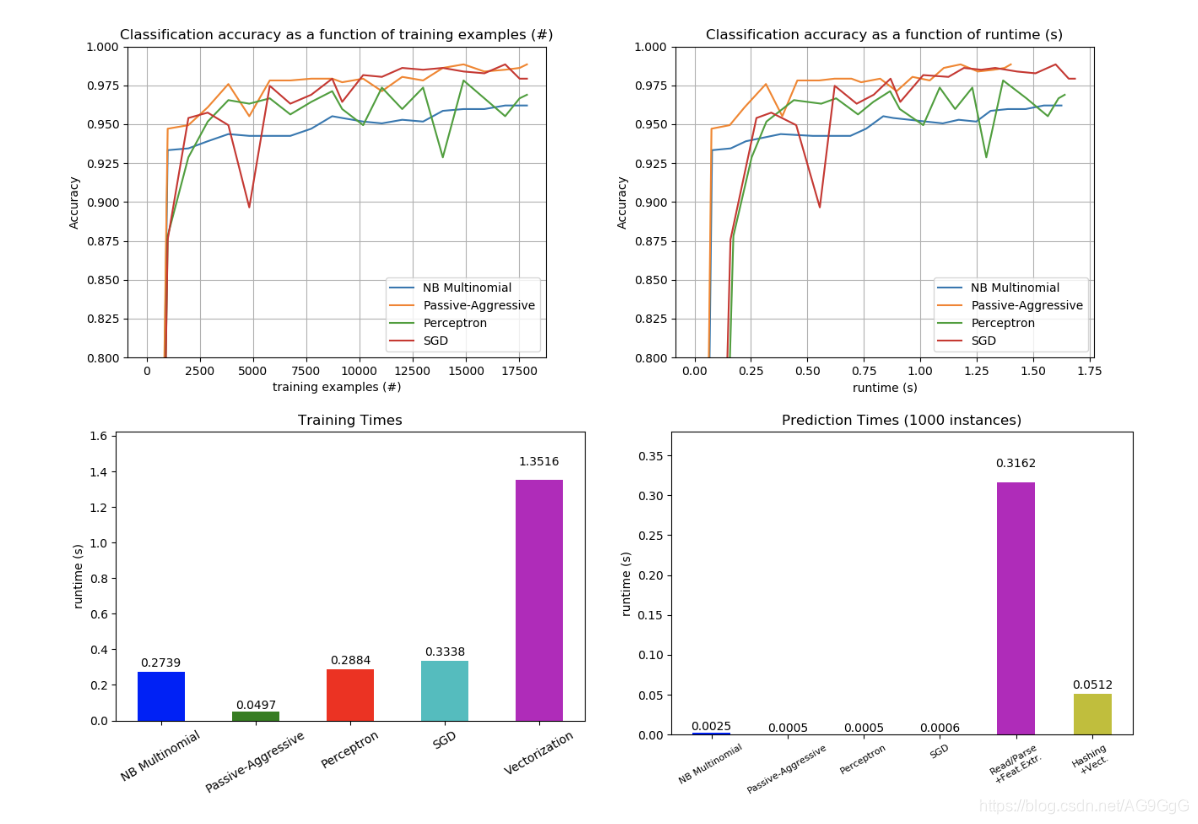
将训练结果可视化
def plot_accuracy(x, y, x_legend):
    """Plot accuracy as a function of x."""
    x = np.array(x)
    y = np.array(y)
    plt.title('Classification accuracy as a function of %s' % x_legend)
    plt.xlabel('%s' % x_legend)
    plt.ylabel('Accuracy')
    plt.grid(True)
    plt.plot(x, y)


rcParams['legend.fontsize'] = 10
cls_names = list(sorted(cls_stats.keys()))

# Plot accuracy evolution
plt.figure()
for _, stats in sorted(cls_stats.items()):
    # Plot accuracy evolution with #examples
    accuracy, n_examples = zip(*stats['accuracy_history'])
    plot_accuracy(n_examples, accuracy, "training examples (#)")
    ax = plt.gca()
    ax.set_ylim((0.8, 1))
plt.legend(cls_names, loc='best')

plt.figure()
for _, stats in sorted(cls_stats.items()):
    # Plot accuracy evolution with runtime
    accuracy, runtime = zip(*stats['runtime_history'])
    plot_accuracy(runtime, accuracy, 'runtime (s)')
    ax = plt.gca()
    ax.set_ylim((0.8, 1))
plt.legend(cls_names, loc='best')

# Plot fitting times
plt.figure()
fig = plt.gcf()
cls_runtime = []
for cls_name, stats in sorted(cls_stats.items()):
    cls_runtime.append(stats['total_fit_time'])

cls_runtime.append(total_vect_time)
cls_names.append('Vectorization')
bar_colors = ['b', 'g', 'r', 'c', 'm', 'y']

ax = plt.subplot(111)
rectangles = plt.bar(range(len(cls_names)), cls_runtime, width=0.5,
                     color=bar_colors)

ax.set_xticks(np.linspace(0, len(cls_names) - 1, len(cls_names)))
ax.set_xticklabels(cls_names, fontsize=10)
ymax = max(cls_runtime) * 1.2
ax.set_ylim((0, ymax))
ax.set_ylabel('runtime (s)')
ax.set_title('Training Times')


def autolabel(rectangles):
    """attach some text vi autolabel on rectangles."""
    for rect in rectangles:
        height = rect.get_height()
        ax.text(rect.get_x() + rect.get_width() / 2.,
                1.05 * height, '%.4f' % height,
                ha='center', va='bottom')
        plt.setp(plt.xticks()[1], rotation=30)


autolabel(rectangles)
plt.tight_layout()
plt.show()

# Plot prediction times
plt.figure()
cls_runtime = []
cls_names = list(sorted(cls_stats.keys()))
for cls_name, stats in sorted(cls_stats.items()):
    cls_runtime.append(stats['prediction_time'])
cls_runtime.append(parsing_time)
cls_names.append('Read/Parse\n+Feat.Extr.')
cls_runtime.append(vectorizing_time)
cls_names.append('Hashing\n+Vect.')

ax = plt.subplot(111)
rectangles = plt.bar(range(len(cls_names)), cls_runtime, width=0.5,
                     color=bar_colors)

ax.set_xticks(np.linspace(0, len(cls_names) - 1, len(cls_names)))
ax.set_xticklabels(cls_names, fontsize=8)
plt.setp(plt.xticks()[1], rotation=30)
ymax = max(cls_runtime) * 1.2
ax.set_ylim((0, ymax))
ax.set_ylabel('runtime (s)')
ax.set_title('Prediction Times (%d instances)' % n_test_documents)
autolabel(rectangles)
plt.tight_layout()
plt.show()
文章开头提供的链接网页提供源码文件的下载。