Jan. 14 - Jan. 25th 2019 two weeks paper reading

paper reading list— Image Denoising

1 A multiscale Image Denoising Algorithm Based on dilated residual Convolution Network link.

1. Dilated filter
2. Multiscale convolution group

2 Dilated Residual Networks（ResNet）link.

which is the combination of Dilated networks and Residual networks.

2.1 Dilated convolution.

there is a very illustrated explanation about dilated convolution.
link.

2.2 Residual Network

3 Understanding Convolution for semantic segmentationlink.

1. dense upsampling convolution(DUC)
2. bilinear upsampling(interpolation)
3. hybrid dilated convolution(HDC)

4 learning Deep CNN Denoiser Prior for Image restoration(IRCNN)link.

Image restoration(IR)
The object of IR:
y = Hx + v
the purpose of image restoration is to recover the latent clean image x from its
degraded observation y.

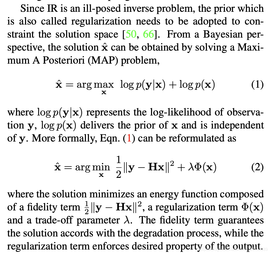
How to solve this type of problem?

1. model-based optimization method
   NCSR, BM3D, WNNM and so on
2. discriminative learning method
   MLP, SRCNN, DCNN and so on
   There are so many different types method of these two classes.
   maybe next time I can give a literature review of these papers.

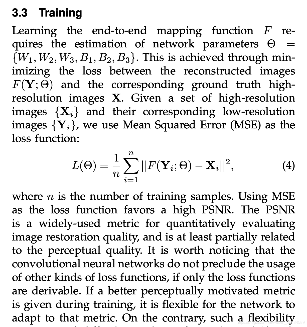
5 Image Super-Resolution Using Deep Convolution Networkslink.

• 5.1 There are 3 steps of this model to improve the performance.

the low-resolution inputs is first upscaled to the desired size using bicubic interpolation before inputing to SRCNN network.

1. Patch Extraction and Representation
   X: Ground truth high-resolution image
   Y: Bicubic upsampling version of low-resolution image
   $F_1(Y) = max(0, W_1 * Y + B_1)$
2. Nonlinear Mapping
   $F_2(Y) = max(0, W_2 * F_1(Y) + B_2)$
3. To Reconstruct the image
   $F(Y) = W_3 * F_2(Y) + B_3$
   $W_3$: $n_2$ * 1 * 1 * C

• 5.2 loss fuction

• 5.3 the limitation of this model (SRCNN)

1. rely on the context of small image regions
2. the training converge too slowly
3. network only works for a single scale

6. Accurate Image Super- Resolution using Very Deep Convolution Networks(VDSR) link.

HR high- resolution
LR low-resolution

• 6.1 innovation point

1. context: very deep network using large receptive field and take a large image context into account.

• using interpolated low-resolution image as input, and predict the image details.
• we pad zeros before convolutions to keep the size of our feature maps the same.

2. convergence: using residual-learning CNN to speed up the training
   
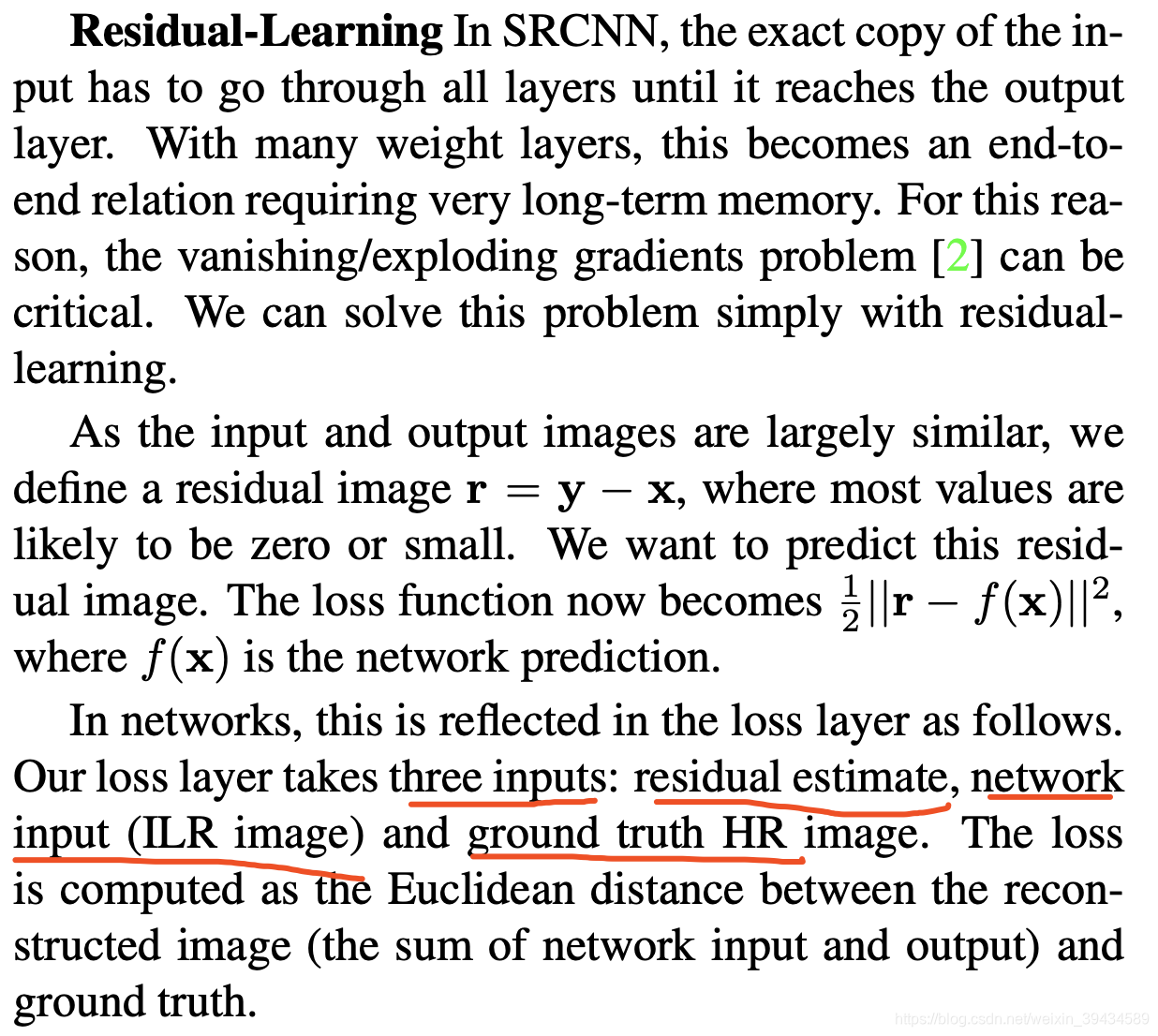
3. scale factor: we propose a single-model SR approach. Scales are typically user-specified and can be arbitrary including fractions.

7 Centralized Sparse representation for Image restoration link.

7.1 Introduction

y = Hx + v
H: degradation matrix
y: observed image
v: additive noise vector
x: original image
x can be represented as a linear combination of a few atoms from a dictionary $\Phi$

x $\approx$ $\Phi$ $\alpha$
$\alpha_x$ = $argmin_\alpha$ $\Vert \alpha \Vert_0$; s.t. $\Vert$ x- $\Phi$ $\alpha$ $\Vert$ $_2$ $\lt$ $\varepsilon$

$\varepsilon$: small constant balacing the sparsity and the approximation error.
$\Vert$ $\Vert$ $_0$ counts the number of non-zero coefficients in $\alpha$

To do the image restoration

y = Hx + v
To reconstruct x from y
Since x $\approx \mathbb{\Phi} \alpha$,
y $\approx$ H $\Phi$ $\alpha$

Then:

• $\alpha_y$ = $argmin_\alpha$ $\Vert \alpha \Vert_1$; s.t. $\Vert$ y - H $\Phi$ $\alpha$ $\Vert$ $_2$ $\lt$ $\varepsilon$
• Reconstruct x:
• $\hat x$ = $\Phi$ $\alpha_y$
  But because y is noise corrupted, blurred or incomplete, $\alpha_y$ may deviate much from $\alpha_x$

In this paper

We introduce the concept of sparse coding noise(SCN) to facilitate the discussion of problem.
$v_\alpha = \alpha _x - \alpha _y$
Given the dictionary $\Phi$
$v_x = \hat x -x \approx$ $\Phi$ $\alpha_y$- $\Phi$ $\alpha_x$= $\Phi$ $v_ \alpha$
We proposed centralized sparse representation model to effectively reduce the SCN and then enhance the sparsity based IR performance.

7.2 Centralized sparse representation modeling

7.2.1 The sparse coding noise in image restoration

X $\in$ $\mathbb R$ $^N$: original image
$x_i = R_i X$
$R_i$ (matrix extracting patch $x_i$ from X at location i)
Given dictionary $\Phi$ $\in \mathbb R ^{n \times M}$ $n \lt M$
each patch can be sparsely represented by the set of sparse code $x_i \approx \Phi \alpha_i$

• In the application of IR, x is not available to code, and we only have the degraded observation image y: y = Hx + v
  $\alpha_y$ = $argmin_\alpha${ $\Vert y - H \Phi \alpha \Vert _2 ^2 + \lambda\Vert \alpha \Vert _1$}

• the image then can be reconstructed as: $\hat x = \Phi \alpha_y$

• from the context we mentioned before, we know that $\alpha_y$ will deviate from $\alpha_x$

• So that SCN : $v_\alpha =\alpha_y -\alpha_x$ And $v_\alpha$ will determine the IR quality of $\hat x$

• We perform the experiment to investigate the statistics of SCN $v_\alpha$, And the observation motivate us to model SCN with a laplacian prior.
  Laplacian distribution $f(x) = \frac{1}{2b} exp(\frac{ - \vert x -\nu \vert}{b})$

7.2.2 Centralized sparse representation

From the context we have mentioned before, we know that if we want to improve the performance of the model, we need to suppress the SCN : $v_\alpha$
$v_\alpha = \alpha_y -\alpha_x$
But in practice, $\alpha_x$ is always unknown, so we can give a good estimate of $\alpha_x$, donated as $\hat \alpha_x$, so that $\alpha_y - \hat \alpha_x$ can be an estimate of SCN.

• A new sparse coding model can be:
• $\alpha_y$ = $argmin_\alpha${ $\Vert y - H \Phi \alpha \Vert _2 ^2 + \lambda\Vert \alpha \Vert _1$+ r $\Vert$ $\alpha$ - $\hat \alpha_x$ $\Vert$ $_{l_p}$}
  r is constant
  ${l_p}$ norm, p can be 1 OR 2 measure the distance between $\alpha$ and $\hat \alpha_x$
• Compared with the model before, this model enforce $\alpha_y$ to be more close to $\hat \alpha_x$.

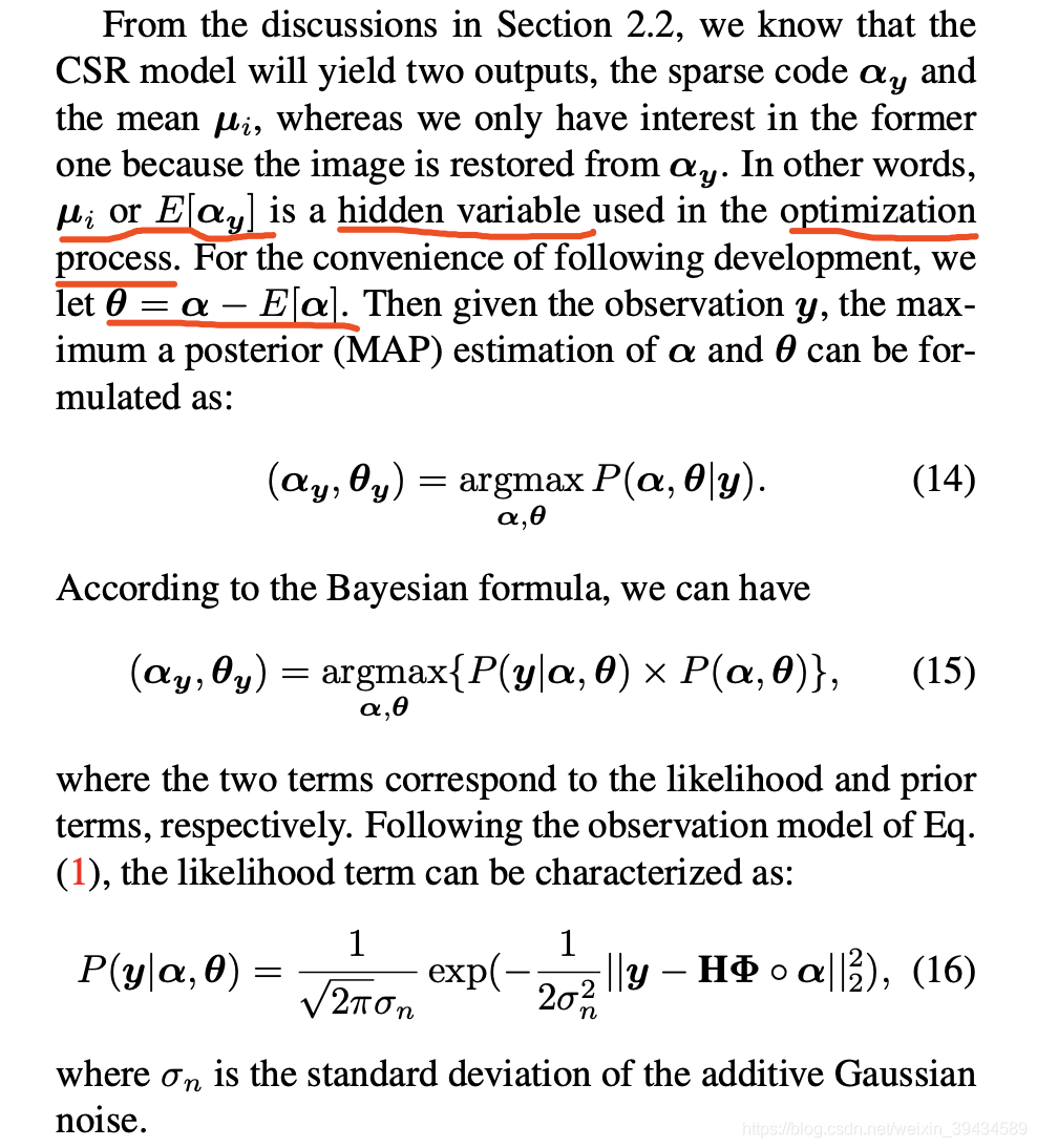
Now the problem turn to be how to find a reasonable estimate of the unknown vector $\alpha_x$

Normally, the estimate of a variable can be the average of several samples or the expectation.
In this part, we use expectation to estimate the $\alpha_x$.
$\hat \alpha_x$ = E[ $\alpha_x$], and in practice, we can approach E[ $\alpha_x$] by E[ $\alpha_y$], by assuming the SCN is nearly zero.

• Then the model we have showed before can be:
• • $\alpha_y$ = $argmin_\alpha${ $\Vert y - H \Phi \alpha \Vert _2 ^2 + \lambda\Vert \alpha \Vert _1$+ r $\Vert$ $\alpha$ - E[ $\alpha$] $\Vert$ $_{l_p}$}
• We call this model centralized sparse representation (CSR)
• For the sparse code $\alpha_i$ on each image patch i, E[ $\alpha_i$] can be nearly computed if we have enough samples of $\alpha_i$. Then E[ $\alpha_i$] can be computed as the weighted average of those sparse code vectors associated with the nonlocal similar patches to patch i. Donated $C_i$ for each patch i via block matching and then average the sparse codes within each cluster.
• Denoted by $\alpha_{i,j}$, the sparse code of the searched similar patch j to patch i.
• Then E[ $\alpha_i$] = $u_i$ = $\sum _{j\in C_i} \omega_{i,j} \alpha_{i,j}$
• $\omega_{i,j}$ is the weight
  $\omega_{i,j} = exp(\Vert \hat {x_i} - \hat {x_{i,j}} \Vert _2 ^2/h)/W$
  $\hat {x_i} = \Phi \hat \alpha_i$; $\hat {x_{i,j}} = \Phi \hat \alpha_{i,j}$ are the estimate of patch i and patch j. W is the normalization factor and h is predetermined scalar.
• $\alpha_y$ = $argmin_\alpha${ $\Vert y - H \Phi \alpha \Vert _2 ^2 + \lambda\Vert \alpha \Vert _1$+ r $\sum_{i =1}^{N}$ $\Vert$ $\alpha_i$ - $u_i$ $\Vert$ $_{l_p}$}

Then we can apply iterative minimization approach to the CSR model.

The steps are as follows:

1. initialize $u_i$ as 0, eg: $u_i ^{(-1)} =0$ Then compute $\alpha_y ^{(0)}$, and then, using $\alpha_y ^{(0)}$, we can compute $x^{(0)}$ via $x^{(0)}=\Phi \alpha_y ^{(0)}$.
2. Based on $x^{(0)}$, we can find the similar patches with each local patch i, then we can update $u_i$ by $\alpha_y ^{(0)}$, and the updated result, donated by $u_i^{0}$. Then it can be used in next round. Such a procedure is iterated until convergence. In the $j^{th}$ iteration, the sparse coding is performed by.
   $\alpha_y^{(j)}$ = $argmin_\alpha${ $\Vert y - H \Phi \alpha \Vert _2 ^2 + \lambda\Vert \alpha \Vert _1$+ r $\sum_{i =1}^{N}$ $\Vert$ $\alpha_i$ - $u_i^{(j)}$ $\Vert$ $_{l_p}$}

During iteration, the accuracy of sparse code $\alpha_y ^{(j)}$ is gradually improved.

7.3 Algorithm of CSR

7.3.1 The determination of parameters $\lambda$ and r.

It can be empirically found that $\alpha$ and $\theta$ are nearly uncorrelated.
And before we have found that SCN can be well characterized by the laplacian distribution.
Meanwhile, it is also well accepted in literature that the sparse coefficients $\alpha$ can be characterized by i.i.d Laplacian distribution.

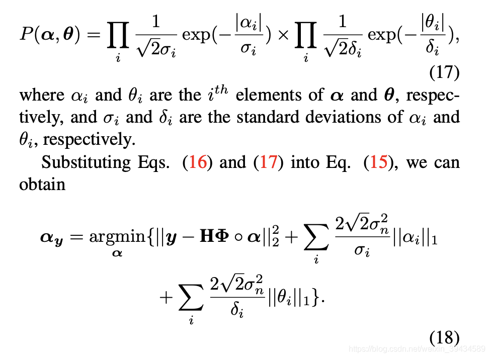
$\alpha_y$ = $argmin_\alpha${ $\Vert y - H \Phi \alpha \Vert _2 ^2 + \lambda\Vert \alpha \Vert _1$+ r $\sum_{i =1}^{N}$ $\Vert$ $\alpha_i$ - $u_i$ $\Vert$ $_{l_p}$}

It is normally for us to set $l_p$ equal to 1
And then the model can be converted to:

$\alpha_y$ = $argmin_\alpha${ $\Vert y - H \Phi \alpha \Vert _2 ^2 + \lambda\Vert \alpha \Vert _1$+ r $\sum_{i =1}^{N}$ $\Vert$ $\alpha_i$ - $u_i$ $\Vert$ $_{1}$}
$\alpha_y$ = $argmin_\alpha${ $\Vert y - H \Phi \alpha \Vert _2 ^2 + \lambda$ $\sum_{i =1}^{N}$ $\Vert$ $\alpha_i \Vert _1$+ r $\sum_{i =1}^{N}$ $\Vert$ $\theta_i$ $\Vert$ $_{1}$}

Compared this model with eq(18)
we can conclude that:

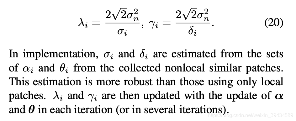
This is the end of this model.