【论文复现】使用CNN进行文本分类

写在前面

不想做实验，不想看算法，不想刷Leetcode，只想躺尸，，，

每天都会有这样的想法，嗯，想想就好了。

最近看概率图这一块看得头疼，算了吧，不如写一写blog。

跟着大牛们的论文复现代码，然后一点一点学习吧。嗯

今天要写的是关于NLP领域的一个关键问题：文本分类。

相对应的论文是：Convolutional Neural Networks for Sentence Classification

全部的代码github：text classification using cnn

NLP中的CNN

论文中是使用的CNN框架来实现对句子的分类，积极或者消极。当然这里我们首先必须对CNN有个大概的了解，可以参考我之前的这篇【Deep learning】卷积神经网络CNN结构。目前主流来看，CNN主要是应用在computer vision领域，并且可以说由于CNN的出现，是的CV的研究与应用都有了质的飞跃。（可惜的是，目前在NLP领域还没有这种玩意儿，不知道刚出的BERT算不算）

目前对NLP的研究分析应用最多的就是RNN系列的框架，比如RNN,GRU,LSTM等等，再加上Attention，基本可以认为是NLP的标配套餐了。但是在文本分类问题上，相比于RNN，CNN的构建和训练更为简单和快速，并且效果也不差，所以仍然会有一些研究。

那么，CNN到底是怎么应用到NLP上的呢？

不同于CV输入的图像像素，NLP的输入是一个个句子或者文档。句子或文档在输入时经过embedding（word2vec或者Glove）会被表示成向量矩阵，其中每一行表示一个词语，行的总数是句子的长度，列的总数就是词表的长度。例如一个包含十个词语的句子，使用了100维的embedding，最后我们就有一个输入为10x100的矩阵。

在CV中，filters是以一个patch（任意长度x任意宽度）的形式滑过遍历整个图像，但是在NLP中，filters会覆盖到所有的词表长度，也就是形状为 [filter_size, vocabulary_size]。更为具体地理解可以看下图，输入为一个7x5的矩阵，filters的高度分别为2,3,4，宽度和输入矩阵一样为5。每个filter对输入矩阵进行卷积操作得到中间特征，然后通过pooling提取最大值，最终得到一个包含6个值的特征向量。

弄清楚了CNN的结构，下面就可以开始实现文本分类任务了。

数据预处理

原论文中使用了好几个数据集，这里我们只选择其中的一个——Movie Review Data from Rotten Tomatoes。该数据集包括了10662个评论，其中一半positive一般negative。

在数据处理阶段，主要包括以下几个部分：

1、load file

def load_data_and_labels(positive_file, negative_file):
    #load data from files
    positive_examples = list(open(positive_file, "r", encoding='utf-8').readlines())
    positive_examples = [s.strip() for s in positive_examples]
    negative_examples = list(open(negative_file, "r", encoding='utf-8').readlines())
    negative_examples = [s.strip() for s in negative_examples]
    # Split by words
    x_text = positive_examples + negative_examples
    x_text = [clean_str(sent) for sent in x_text]
    # Generate labels
    positive_labels = [[0, 1] for _ in positive_examples]
    negative_labels = [[1, 0] for _ in negative_examples]
    y = np.concatenate([positive_labels, negative_labels], 0)
    return [x_text, y]

2、clean sentences

def clean_str(string):
    string = re.sub(r"[^A-Za-z0-9(),!?\'\`]", " ", string)
    string = re.sub(r"\'s", " \'s", string)
    string = re.sub(r"\'ve", " \'ve", string)
    string = re.sub(r"n\'t", " n\'t", string)
    string = re.sub(r"\'re", " \'re", string)
    string = re.sub(r"\'d", " \'d", string)
    string = re.sub(r"\'ll", " \'ll", string)
    string = re.sub(r",", " , ", string)
    string = re.sub(r"!", " ! ", string)
    string = re.sub(r"\(", " \( ", string)
    string = re.sub(r"\)", " \) ", string)
    string = re.sub(r"\?", " \? ", string)
    string = re.sub(r"\s{2,}", " ", string)
    return string.strip().lower()

模型实现

论文中使用的模型如下所示

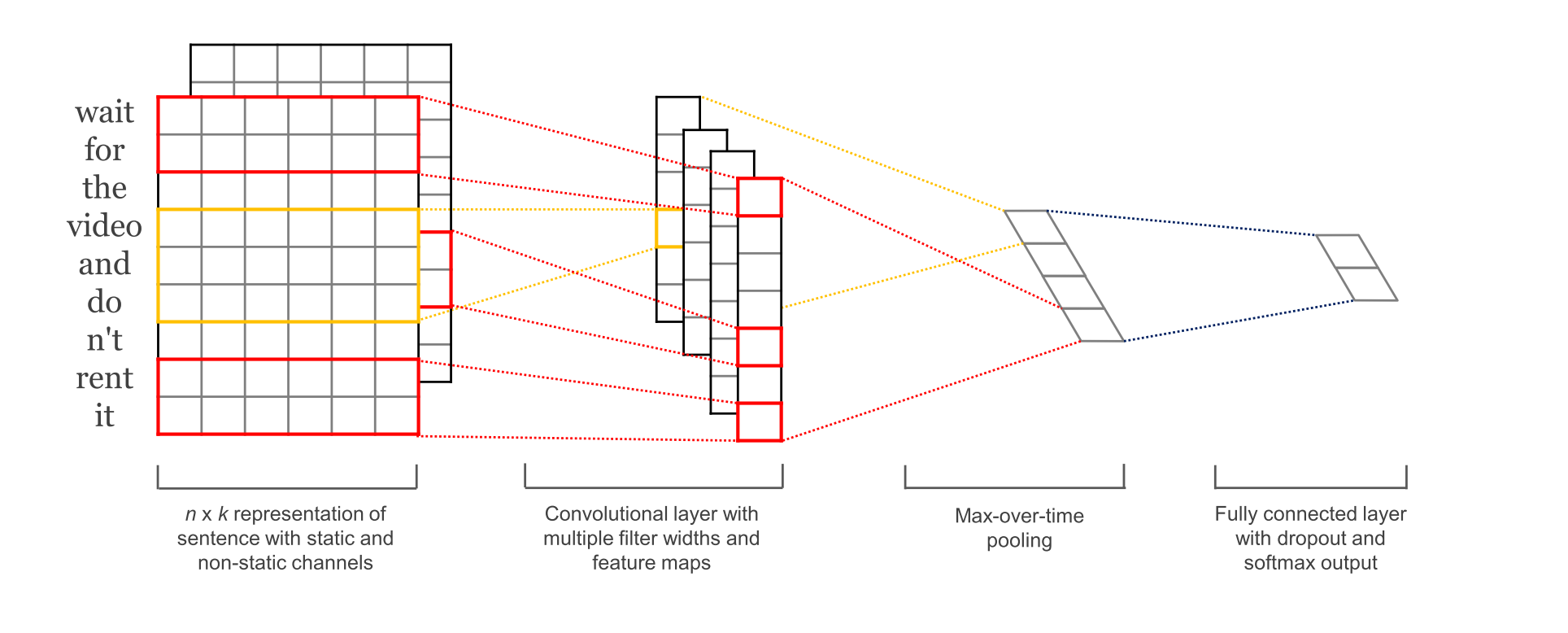
其中第一层为embedding layer，用于把单词映射到一组向量表示。接下去是一层卷积层，使用了多个filters，这里有3,4,5个单词一次遍历。接着是一层max-pooling layer 得到了一列长特征向量，然后在dropout 之后使用softmax得出每一类的概率。

在一个CNN类中实现上述模型

class TextCNN(object):
    """
    A CNN class for sentence classification
    With a embedding layer + a convolutional, max-pooling and softmax layer
    """
    def __init__(self, sequence_length, num_classes, vocab_size,
                 embedding_size, filter_sizes, num_filters, l2_reg_lambda=0.0):
        """

        :param sequence_length: The length of our sentences
        :param num_classes:     Number of classes in the output layer(pos and neg)
        :param vocab_size:      The size of our vocabulary
        :param embedding_size:  The dimensionality of our embeddings.
        :param filter_sizes:    The number of words we want our convolutional filters to cover
        :param num_filters:     The number of filters per filter size
        :param l2_reg_lambda:   optional

这里再注释一下filter_sizes和num_filters。filters_sizes是指filter每次处理几个单词，num_filters是指每个尺寸的处理包含几个filter。

Input placeholder

tf.placeholder是tensorflow的一种占位符，与feeed_dict同时使用。在训练或者测试模型阶段，我们可以通过feed_dict来喂入输入变量。

# set placeholders for variables
self.input_x = tf.placeholder(tf.int32, [None, sequence_length], name='input_x')
self.input_y = tf.placeholder(tf.float32, [None, num_classes], name='input_y')
self.dropout_keep_prob = tf.placeholder(tf.float32, name='dropout_keep_prob')

tf.placeholder函数第一个参数是变量类型，第二个参数是变量shape，其中None表示sample的个数，第三个name参数用于指定名字。

dropout_keep_prob变量是在dropout阶段使用的，我们在训练的时候选取50%的dropout，在测试时不适用dropout。

Embedding layer

我们需要定义的第一个层是embedding layer，用于将词语转变成为一组向量表示。

 # embedding layer
 with tf.name_scope('embedding'):
        self.W = tf.Variable(tf.random_uniform([vocab_size, embedding_size], -1.0, 1.0), name='weight')
        self.embedded_chars = tf.nn.embedding_lookup(self.W, self.input_x)
        # TensorFlow’s convolutional conv2d operation expects a 4-dimensional tensor
        # with dimensions corresponding to batch, width, height and channel.
        self.embedded_chars_expanded = tf.expand_dims(self.embedded_chars, -1)

W 是在训练过程中学习到的参数矩阵，然后通过tf.nn.embedding_lookup来查找到与input_x相对应的向量表示。tf.nn.embedding_lookup返回的结果是一个三维向量，[None, sequence_length, embedding_size]。但是后一层的卷积层要求输入为四维向量（batch， width，height，channel）。所以我们要将结果扩展一个维度，才能符合下一层的输入。

Convolution and Max-Pooling Layers

在卷积层中最重要的就是filter。回顾本文的第一张图，我们一共有三种类型的filter，每种类型有两个。我们需要迭代每个filter去处理输入矩阵，将最终得到的所有结果合并为一个大的特征向量。

# conv + max-pooling for each filter
        pooled_outputs = []
        for i, filter_size in enumerate(filter_sizes):
            with tf.name_scope('conv-maxpool-%s' % filter_size):
                # conv layer
                filter_shape = [filter_size, embedding_size, 1, num_filters]
                W = tf.Variable(tf.truncated_normal(filter_shape, stddev=0.1), name='W')
                b = tf.Variable(tf.constant(0.1, shape=[num_filters]), name='b')
                conv = tf.nn.conv2d(self.embedded_chars_expanded, W, strides=[1,1,1,1],
                                    padding='VALID', name='conv')
                # activation
                h = tf.nn.relu(tf.nn.bias_add(conv, b), name='relu')
                # max pooling
                pooled = tf.nn.max_pool(h, ksize=[1, sequence_length-filter_size + 1, 1, 1],
                                        strides=[1,1,1,1], padding='VALID', name='pool')
                pooled_outputs.append(pooled)


        # combine all the pooled fratures
        num_filters_total = num_filters * len(filter_sizes)
        self.h_pool = tf.concat(pooled_outputs, 3)  # why 3?
        self.h_pool_flat = tf.reshape(self.h_pool, [-1, num_filters_total])

这里W 就是filter矩阵， tf.nn.conv2d是tensorflow的卷积操作函数，其中几个参数包括

strides表示每一次filter滑动的距离，它总是一个四维向量，而且首位和末尾必定要是1，[1, width, height, 1]。

padding有两种取值：VALID和SAME。VALID是指不在输入矩阵周围填充0，最后得到的output的尺寸小于input；

SAME是指在输入矩阵周围填充0，最后得到output的尺寸和input一样；

这里我们使用的是‘VALID’，所以output的尺寸为[1, sequence_length - filter_size + 1, 1, 1]。

接下去是一层max-pooling，pooling比较好理解，就是选出其中最大的一个。经过这一层的output尺寸为 [batch_size, 1, 1, num_filters]。

Dropout layer

这个比较好理解，就是为了防止模型的过拟合，设置了一个神经元激活的概率。每次在dropout层设置一定概率使部分神经元失效，每次失效的神经元都不一样，所以也可以认为是一种bagging的效果。

# dropout
        with tf.name_scope('dropout'):
            self.h_drop = tf.nn.dropout(self.h_pool_flat, self.dropout_keep_prob)

Scores and Predictions

我们可以通过对上述得到的特征进行运算得到每个分类的分数score，并且可以通过softmax将score转化成概率分布，选取其中概率最大的一个作为最后的prediction

#score and prediction
        with tf.name_scope("output"):
            W = tf.get_variable('W', shape=[num_filters_total, num_classes],
                                initializer = tf.contrib.layers.xavier_initializer())
            b = tf.Variable(tf.constant(0.1, shape=[num_classes]), name='b')
            l2_loss += tf.nn.l2_loss(W)
            l2_loss += tf.nn.l2_loss(b)
            self.score = tf.nn.xw_plus_b(self.h_drop, W, b, name='scores')
            self.prediction = tf.argmax(self.score, 1, name='prediction')

Loss and Accuracy

通过score我们可以计算得出模型的loss，而我们训练的目的就是最小化这个loss。对于分类问题，最常用的损失函数是cross-entropy 损失

 # mean cross-entropy loss
        with tf.name_scope('loss'):
            losses = tf.nn.softmax_cross_entropy_with_logits(logits=self.score, labels=self.input_y)
            self.loss = tf.reduce_mean(losses) + l2_reg_lambda * l2_loss

为了在训练过程中实时观测训练情况，我们可以定义一个准确率

# accuracy
        with tf.name_scope('accuracy'):
            correct_predictions = tf.equal(self.prediction, tf.argmax(self.input_y, 1))
            self.accuracy = tf.reduce_mean(tf.cast(correct_predictions, 'float'), name='accuracy')

到目前为止，我们的模型框架已经搭建完成，可以使用Tensorboardd来瞧一瞧到底是个啥样

接下去我们就要开始使用影评数据来训练网络啦。

Training procedure

对于Tensorflow有两个重要的概念：Graph和Session。

Session会话可以理解为一个计算的环境，所有的operation只有在session中才能返回结果；

Graph图就可以理解为上面那个图片，在图里面包含了所有要用到的操作operations和张量tensors。

PS：在一个项目中可以使用多个graph，不过我们一般习惯只用一个就行。同时，在一个graph中可以有多个session，但是在一个session中不能有多个graph。

    with tf.Graph().as_default():
        session_conf = tf.ConfigProto(
            # allows TensorFlow to fall back on a device with a certain operation implemented
            allow_soft_placement= FLAGS.allow_soft_placement,
            # allows TensorFlow log on which devices (CPU or GPU) it places operations
            log_device_placement=FLAGS.log_device_placement
        )
        sess = tf.Session(config=session_conf)

Instantiating the CNN and minimizing the loss

# initialize cnn
cnn = TextCNN(sequence_length=x_train.shape[1],
              num_classes=y_train.shape[1],
              vocab_size= len(vocab_processor.vocabulary_),
              embedding_size=FLAGS.embedding_dim,
              filter_sizes= list(map(int, FLAGS.filter_sizes.split(','))),
              num_filters= FLAGS.num_filters,
              l2_reg_lambda= FLAGS.l2_reg_lambda)

global_step = tf.Variable(0, name='global_step', trainable=False)
optimizer = tf.train.AdamOptimizer(1e-3)
grads_and_vars = optimizer.compute_gradients(cnn.loss)
train_op = optimizer.apply_gradients(grads_and_vars, global_step=global_step)

这里train_op的作用就是更新参数，每运行一次train_op，global_step都会增加1。

Summaries

Tensorflow有一个特别实用的操作，summary，它可以记录训练时参数或者其他变量的变化情况并可视化到tensorboard。使用tf.summary.FileWriter()函数可以将summaries写入到硬盘保存到本地。

# visualise gradient
            grad_summaries = []
            for g, v in grads_and_vars:
                if g is not None:
                    grad_hist_summary = tf.summary.histogram('{}/grad/hist'.format(v.name),g)
                    sparsity_summary = tf.summary.scalar('{}/grad/sparsity'.format(v.name), tf.nn.zero_fraction(g))
                    grad_summaries.append(grad_hist_summary)
                    grad_summaries.append(sparsity_summary)
            grad_summaries_merged = tf.summary.merge(grad_summaries)

            # output dir for models and summaries
            timestamp = str(time.time())
            out_dir = os.path.abspath(os.path.join(os.path.curdir, 'run', timestamp))
            print('Writing to {} \n'.format(out_dir))

            # summaries for loss and accuracy
            loss_summary = tf.summary.scalar('loss', cnn.loss)
            accuracy_summary = tf.summary.scalar('accuracy', cnn.accuracy)

            # train summaries
            train_summary_op = tf.summary.merge([loss_summary, accuracy_summary])
            train_summary_dir = os.path.join(out_dir, 'summaries', 'train')
            train_summary_writer = tf.summary.FileWriter(train_summary_dir, sess.graph)

            # dev summaries
            dev_summary_op = tf.summary.merge([loss_summary, accuracy_summary])
            dev_summary_dir = os.path.join(out_dir, 'summaries', 'dev')
            dev_summary_writer = tf.summary.FileWriter(dev_summary_dir, sess.graph)

Checkpointing

checkpointing的作用就是可以保存每个阶段训练模型的参数，然后我们可以根据准确率来选取最好的一组参数。

# checkpoint dir. checkpointing – saving the parameters of your model to restore them later on.
            checkpoint_dir = os.path.abspath(os.path.join(out_dir, 'checkpoints'))
            checkpoint_prefix = os.path.join(checkpoint_dir, 'model')
            if not os.path.exists(checkpoint_dir):
                os.makedirs(checkpoint_dir)
            saver = tf.train.Saver(tf.global_variables(), max_to_keep=FLAGS.num_checkpoints)

Initializing the variables

在开始训练之前，我们通常会需要初始化所有的变量

一般使用 tf.global_variables_initializer()就可以了。

Defining a single training step

我们可以定义一个单步训练的函数，使用一个batch的数据来更新模型的参数

            def train_step(x_batch, y_batch):
                """
                A single training step
                :param x_batch:
                :param y_batch:
                :return:
                """
                feed_dict = {
                    cnn.input_x: x_batch,
                    cnn.input_y: y_batch,
                    cnn.dropout_keep_prob: FLAGS.dropout_keep_prob
                }
                _, step, summaries, loss, accuracy = sess.run(
                    [train_op, global_step, train_summary_op, cnn.loss, cnn.accuracy],
                    feed_dict=feed_dict
                )
                time_str = datetime.datetime.now().isoformat()
                print("{}: step {}, loss {:g}, acc {:g}".format(time_str, step, loss, accuracy))
                train_summary_writer.add_summary(summaries, step)

这里的feed_dict就是我们前面提到的同placeholder一起使用的。必须在feed_dict中给出说有placeholder节点的值，否则程序就会报错。

接着使用sess.run（）运行前面定义的操作，最终可以得到每一步的损失、准确率这些信息。

类似地我们定义一个函数在验证集数据上看看模型的准确率等

            def dev_step(x_batch, y_batch, writer=None):
                """
                Evaluate model on a dev set
                Disable dropout
                :param x_batch:
                :param y_batch:
                :param writer:
                :return:
                """
                feed_dict = {
                    cnn.input_x: x_batch,
                    cnn.input_y: y_batch,
                    cnn.dropout_keep_prob: 1.0
                }
                step, summaries, loss, accuracy = sess.run(
                    [global_step, dev_summary_op, cnn.loss, cnn.accuracy],
                    feed_dict=feed_dict
                )
                time_str = datetime.datetime.now().isoformat()
                print("{}: step {}, loss {:g}, acc {:g}".format(time_str, step, loss, accuracy))
                if writer:
                    writer.add_summary(summaries, step)

Training loop

前面都定义好了以后就可以开始我们的训练了。我们每次调用train_step函数批量的训练数据并保存：

# generate batches
            batches = data_process.batch_iter(list(zip(x_train, y_train)), FLAGS.batch_size, FLAGS.num_epochs)
            # training loop
            for batch in batches:
                x_batch, y_batch = zip(*batch)
                train_step(x_batch, y_batch)
                current_step = tf.train.global_step(sess, global_step)
                if current_step % FLAGS.evaluate_every == 0:
                    print('\n Evaluation:')
                    dev_step(x_dev, y_dev, writer=dev_summary_writer)
                    print('')
                if current_step % FLAGS.checkpoint_every == 0:
                    path = saver.save(sess, checkpoint_prefix, global_step=current_step)
                    print('Save model checkpoint to {} \n'.format(path))

最后输出的效果大概是这样的

Visualizing Results

我们可以在代码目录下打开终端输入以下代码来启动浏览器的tensorboard：

tensorboard --logdir /runs/xxxxxx/summaries

=======================================================================================================

当然这只是一个利用CNN进行NLP分类任务（文本分类，情感分析等）的baseline，可以看出准确率并不是很高，后续还有很多可以优化的地方，包括使用pre-trained的Word2vec向量、加上L2正则化等等。

以上~