目录
代码运行
代码分析
代码运行
同样分析tensorflow版的实现,代码地址:SSD-Tensorflow
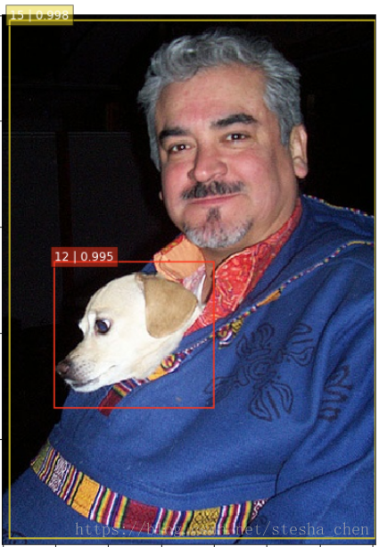
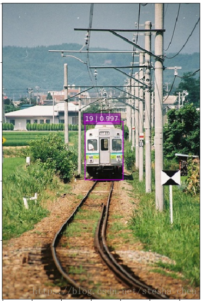
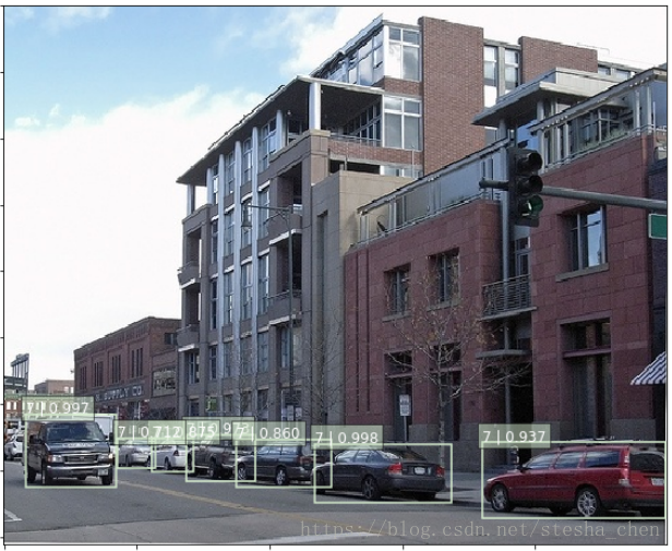
1.预测
unzip ssd_300_vgg.ckpt.zipjupyter notebook notebooks/ssd_notebook.ipynb启动jupyter notebook后,我们运行里面的代码就可以进行预测了。
2.训练
准备数据
首先下载VOC数据,下载方式可以参考https://blog.csdn.net/stesha_chen/article/details/82965283
创建文件夹tfrecords,然后运行tf_convert_data.py,将VOC数据转成tfrecord方式存储,后面会细读这部分的代码。
python tf_convert_data.py \
    --dataset_name=pascalvoc \
    --dataset_dir=./VOCdevkit/VOC2007/ \
    --output_name=voc_2007_train \
    --output_dir=./tfrecords
基于pre-trained VGG
由于SSD网络的base network就是一个分类网络,所以就算是从头开始训练SSD,我们也会先用训练好的分类网络初始化SSD的前面层,这里以VGG为例。
先下载预先训练好的VGG权重文件,VGG下载地址
python train_ssd_network.py \
    --train_dir=./log \
    --dataset_dir=./tfrecords \
    --dataset_name=pascalvoc_2007 \
    --dataset_split_name=train \
    --model_name=ssd_300_vgg \
    --checkpoint_path=./checkpoints/vgg_16.ckpt \
    --checkpoint_model_scope=vgg_16 \
    --checkpoint_exclude_scopes=ssd_300_vgg/conv6,ssd_300_vgg/conv7,ssd_300_vgg/block8,ssd_300_vgg/block9,ssd_300_vgg/block10,ssd_300_vgg/block11,ssd_300_vgg/block4_box,ssd_300_vgg/block7_box,ssd_300_vgg/block8_box,ssd_300_vgg/block9_box,ssd_300_vgg/block10_box,ssd_300_vgg/block11_box \
    --trainable_scopes=ssd_300_vgg/conv6,ssd_300_vgg/conv7,ssd_300_vgg/block8,ssd_300_vgg/block9,ssd_300_vgg/block10,ssd_300_vgg/block11,ssd_300_vgg/block4_box,ssd_300_vgg/block7_box,ssd_300_vgg/block8_box,ssd_300_vgg/block9_box,ssd_300_vgg/block10_box,ssd_300_vgg/block11_box \
    --save_summaries_secs=60 \
    --save_interval_secs=600 \
    --weight_decay=0.0005 \
    --optimizer=adam \
    --learning_rate=0.001 \
    --learning_rate_decay_factor=0.94 \
    --batch_size=32
--train_dir表示训练权重,tensorboard等信息保存的地址
--dataset_dir表示转出来的tfrecords保存的地址
--dataset_name表示我们现在训练哪个数据集,因为不同的数据集,在解析方式上是有些微差别的
--dataset_split_name表示我们现在是用pascalvoc_2007数据集的train数据还是test数据
--model_name表示我们模型的名字,检测模型是SSD,输入是300x300,base network是VGG
--checkpoint_path就是VGG pre-trained weights存放的地址
--checkpoint_exclude_scopes表示这些参数不需要从checkpoint中恢复
--trainable_scopes表示训练的时候只更新这些参数的值
基于pre-trained SSD
在用jupyter运行的时候我们已经将预先训练好的SSD权重文件下载了,运行下面的命令就可以继续训练了
python train_ssd_network.py \
    --train_dir=./log/ \
    --dataset_dir=./tfrecords \
    --dataset_name=pascalvoc_2007 \
    --dataset_split_name=train \
    --model_name=ssd_300_vgg \
    --checkpoint_path=./checkpoints/ssd_300_vgg.ckpt \
    --save_summaries_secs=60 \
    --save_interval_secs=600 \
    --weight_decay=0.0005 \
    --optimizer=adam \
    --learning_rate=0.001 \
    --batch_size=32
3.评估
python eval_ssd_network.py \
    --eval_dir=./log/eval \
    --dataset_dir=./tfrecords \
    --dataset_name=pascalvoc_2007 \
    --dataset_split_name=test \
    --model_name=ssd_300_vgg \
    --checkpoint_path=./checkpoints/ssd_300_vgg.ckpt \
    --wait_for_checkpoints=True \
    --batch_size=1 \
    --max_num_batches=500
代码分析
数据准备
在tf_convert_data.py中主要是调用了pascalvoc_to_tfrecords.run,第一个参数dataset_dir是./VOCdevkit/VOC2007,第二个参数output_dir是./tfrecords,第三个参数是voc_2007_train
    path = os.path.join(dataset_dir, DIRECTORY_ANNOTATIONS)
    filenames = sorted(os.listdir(path))
path是./VOCdevkit/VOC2007/Annotations,列出里面的所有文件就是filenames,每个文件是对图片进行标记的xml文件。
然后遍历所有文件,将200个文件放入一条tfrecord记录中。
        # 创建TFRecordWriter
        with tf.python_io.TFRecordWriter(tf_filename) as tfrecord_writer:
            j = 0
            # 循环200次放入同一条tfrecord中
            while i < len(filenames) and j < SAMPLES_PER_FILES:
                filename = filenames[i]
                img_name = filename[:-4]
                # 将数据写入tfrecord中
_add_to_tfrecord(dataset_dir, img_name, tfrecord_writer)在_add_to_tfrecord函数中先调用_process_image对数据进行解析,返回值如下:
image_data是通过tf.gfile.FastGFile(filename, 'r').read()读出来的图片buffer
    filename = directory + DIRECTORY_IMAGES + name + '.jpg'
image_data = tf.gfile.FastGFile(filename, 'r').read()shape是从xml中读出的size信息
    shape = [int(size.find('height').text),
             int(size.find('width').text),
int(size.find('depth').text)]bboxes是从xml中读出的每个物体的位置框,如果图片中两个物体那么bboxes的长度为2,里面放着两个bbox信息
        bbox = obj.find('bndbox')
        bboxes.append((float(bbox.find('ymin').text) / shape[0],
                       float(bbox.find('xmin').text) / shape[1],
                       float(bbox.find('ymax').text) / shape[0],
                       float(bbox.find('xmax').text) / shape[1]
))labels中保存一张图片上所有物体对应的id,比如图片上有dog和bird,那么labels=[12, 3]
        label = obj.find('name').text
labels.append(int(VOC_LABELS[label][0]))labels_text中保存一张图片中所有物体的名字
        label = obj.find('name').text
labels_text.append(label.encode('ascii'))difficult中保存所有物体是否是difficult的参数,如果有取其值,如果没有这个参数就设置为0,这个参数表示这个数据是否难标记的,后面对数据集处理的时候可以选择是否过滤掉这部分数据。
        if obj.find('difficult'):
            difficult.append(int(obj.find('difficult').text))
        else:
difficult.append(0)truncated中保存所有物体是否是truncated的参数,如果有取其值,如果没有这个参数就设置为0
        if obj.find('truncated'):
            truncated.append(int(obj.find('truncated').text))
        else:
truncated.append(0)接着在_add_to_tfrecord函数中调用_convert_to_example生成example,传入参数就是我们前面拿到的返回值,xmin是图片中所有物体的xmin的集合,xmax,ymin,ymax同样。
    example = tf.train.Example(features=tf.train.Features(feature={
            'image/height': int64_feature(shape[0]),
            'image/width': int64_feature(shape[1]),
            'image/channels': int64_feature(shape[2]),
            'image/shape': int64_feature(shape),
            'image/object/bbox/xmin': float_feature(xmin),
            'image/object/bbox/xmax': float_feature(xmax),
            'image/object/bbox/ymin': float_feature(ymin),
            'image/object/bbox/ymax': float_feature(ymax),
            'image/object/bbox/label': int64_feature(labels),
            'image/object/bbox/label_text': bytes_feature(labels_text),
            'image/object/bbox/difficult': int64_feature(difficult),
            'image/object/bbox/truncated': int64_feature(truncated),
            'image/format': bytes_feature(image_format),
            'image/encoded': bytes_feature(image_data)}))
最后在_add_to_tfrecord函数中将example写入tfrecord
tfrecord_writer.write(example.SerializeToString())总结一下生成tfrecord只需要如下几步
- tfrecord_writer = tf.python_io.TFRecordWriter(...)
- 解析xml和图片文件
- example = tf.train.Example(...)
- tfrecord_write.write(example.SerializeToString())
基于VGG从头开始训练
训练的入口在train_ssd_network.py中,从main函数开始运行。
1.准备
        # 初始化DeploymentConfig对象,将参数的信息保存在对象中
        # 主要就是配置多GPU的情况,配置是否在CPU上做拷贝等
        # Args:
        #   num_clones: Number of model clones to deploy in each replica.
        #   clone_on_cpu: If True clones would be placed on CPU.
        #   replica_id: Integer.  Index of the replica for which the model is
        #       deployed.  Usually 0 for the chief replica.
        #   num_replicas: Number of replicas to use.
        #   num_ps_tasks: Number of tasks for the `ps` job. 0 to not use replicas.
        deploy_config = model_deploy.DeploymentConfig(
            num_clones=FLAGS.num_clones,
            clone_on_cpu=FLAGS.clone_on_cpu,
            replica_id=0,
            num_replicas=1,
            num_ps_tasks=0)
        # deploy_config.variables_device()就是/device:CPU:0表示下面的参数放在CPU上
        with tf.device(deploy_config.variables_device()):
            # global_step打印出来就是<tf.Variable 'global_step:0' shape=() dtype=int64_ref>
            # 代表全局步数,后面会用到
            global_step = slim.create_global_step()
2.取出dataset
        dataset = dataset_factory.get_dataset(
            FLAGS.dataset_name, FLAGS.dataset_split_name, FLAGS.dataset_dir)
get_dataset最后会调用到pascalvoc_common.py中的get_split来读取tfrecord创建dataset。
首先创建reader
    if reader is None:
        reader = tf.TFRecordReader
然后生成decoder
    decoder = slim.tfexample_decoder.TFExampleDecoder(
        keys_to_features, items_to_handlers)
最后返回由这些参数组成的dataset
    return slim.dataset.Dataset(
            data_sources=file_pattern,
            reader=reader,
            decoder=decoder,
            num_samples=split_to_sizes[split_name],
            items_to_descriptions=items_to_descriptions,
            num_classes=num_classes,
            labels_to_names=labels_to_names)
3.生成anchors
# 现在model_name是ssd_300_vgg,因此ssd_class是ssd_vgg_300.SSDNet
ssd_class = nets_factory.get_network(FLAGS.model_name)
# 等同于调用ssd_vgg_300.SSDNet.default_params._replace
# 也就是调用SSDParams._replace
# 将SSDParams中的num_classes替换成21,不过其实现在就是21
ssd_params = ssd_class.default_params._replace(num_classes=FLAGS.num_classes)
# 就是调用ssd_vgg_300.SSDNet(ssd_params)来生成SSDNet对象
ssd_net = ssd_class(ssd_params)
# ssd_shape是(300, 300)
ssd_shape = ssd_net.params.img_shape
# 调用ssd_anchors_all_layers生成每一层的anchors
ssd_anchors = ssd_net.anchors(ssd_shape)
所以接着看ssd_anchors_all_layers的实现
def ssd_anchors_all_layers(img_shape,
                           layers_shape,
                           anchor_sizes,
                           anchor_ratios,
                           anchor_steps,
                           offset=0.5,
                           dtype=np.float32):
    # img_shape:(300, 300)
    # layers_shape:[(38, 38), (19, 19), (10, 10), (5, 5), (3, 3), (1, 1)]
    # anchor_sizes:[(21., 45.),(45., 99.),(99., 153.),(153., 207.),(207., 261.),(261., 315.)]
    # anchor_ratios:[[2, .5],[2, .5, 3, 1./3],[2, .5, 3, 1./3],[2, .5, 3, 1./3],[2, .5],[2, .5]]
    # anchor_steps:[8, 16, 32, 64, 100, 300]
    # offset:0.5
    layers_anchors = []
    # 跟论文中一样,一共有6层feature map会生成anchors,也就是default box
    # 对每一层feature map生成anchors
    for i, s in enumerate(layers_shape):
        anchor_bboxes = ssd_anchor_one_layer(img_shape, s,
                                             anchor_sizes[i],
                                             anchor_ratios[i],
                                             anchor_steps[i],
                                             offset=offset, dtype=dtype)
        layers_anchors.append(anchor_bboxes)
    return layers_anchors
最后看ssd_anchor_one_layer函数的实现,以第一层(38, 38)为例
def ssd_anchor_one_layer(img_shape,
                         feat_shape,
                         sizes,
                         ratios,
                         step,
                         offset=0.5,
                         dtype=np.float32):
    # img_shape: (300, 300)
    # feat_shape: (38, 38)
    # sizes: (21., 45.)
    # ratios: [2, .5]
    # step: 8
    # x,y是feature map上的每个像素坐标shape=(38, 38)
    y, x = np.mgrid[0:feat_shape[0], 0:feat_shape[1]]
    # 算出xy还原到原图位置后除以输入图片的长宽
    y = (y.astype(dtype) + offset) * step / img_shape[0]
    x = (x.astype(dtype) + offset) * step / img_shape[1]

    # Expand dims to support easy broadcasting.
    # shape=(38, 38, 1)
    y = np.expand_dims(y, axis=-1)
    x = np.expand_dims(x, axis=-1)

    num_anchors = len(sizes) + len(ratios)
    # 用一定的计算方式生成4组h和w
    h = np.zeros((num_anchors, ), dtype=dtype)
    w = np.zeros((num_anchors, ), dtype=dtype)
    # Add first anchor boxes with ratio=1.
    h[0] = sizes[0] / img_shape[0]
    w[0] = sizes[0] / img_shape[1]
    di = 1
    if len(sizes) > 1:
        h[1] = math.sqrt(sizes[0] * sizes[1]) / img_shape[0]
        w[1] = math.sqrt(sizes[0] * sizes[1]) / img_shape[1]
        di += 1
    for i, r in enumerate(ratios):
        h[i+di] = sizes[0] / img_shape[0] / math.sqrt(r)
        w[i+di] = sizes[0] / img_shape[1] * math.sqrt(r)
    return y, x, h, w
其他的feature map同样处理,不过(19, 19)和(10, 10)和(5, 5)的feature map有6个anchors.现在这些anchors长宽都是一样,后面会做尺度压缩。
4.通过provider获取数据
with tf.name_scope(FLAGS.dataset_name + '_data_provider'):
    # 创建获取数据的provider,这种方式读取数据会比普通方式快很多
    # 因为是多个reader,并且在一个queue准备好后就在准备下一个queue
    provider = slim.dataset_data_provider.DatasetDataProvider(
        dataset,
        num_readers=FLAGS.num_readers,
        common_queue_capacity=20 * FLAGS.batch_size,
        common_queue_min=10 * FLAGS.batch_size,
        shuffle=True)
# Get for SSD network: image, labels, bboxes.
# 通过provider可以获取dataset中的数据
[image, shape, glabels, gbboxes] = provider.get(['image', 'shape',
                                                 'object/label',
'object/bbox'])image:存放图片信息和图片格式信息
shape:存放图片的长宽和channel
glabels:图片中所有物体的label id数组
gbboxes:图片中所有物体的box信息
5.预处理取出来的数据
preprocessing_name = FLAGS.preprocessing_name or FLAGS.model_name
image_preprocessing_fn = preprocessing_factory.get_preprocessing(
    preprocessing_name, is_training=True)
......
# ssd_shape是(300, 300)
# 代码中DATA_FORMAT是NCHW表示Channel在最前面,这里我改成了NHWC,影响不大
image, glabels, gbboxes = \
    image_preprocessing_fn(image, glabels, gbboxes,
                           out_shape=ssd_shape,
                           data_format=DATA_FORMAT)
实际上就是调用ssd_vgg_preprocessing.py中的preprocess_for_train函数
# Distort image and bounding boxes.
dst_image = image
# 调用tf.image.sample_distorted_bounding_box为图像生成随机扭曲的边界框,做数据增强
# dst_image是通过生成的边界框截取出来的图像(None, None, 3)
# distort_bbox是新图片在原图片中的边界框(4,)
# bboxes的生成有以下几个步骤
# 1.将原来的bboxes做调整,生成相对新图片的坐标框
# 2.因为有可能截取的新图片使box的大部分内容丢失,如果box丢失的内容超过0.5则抛弃,这样生成了新的bboxes
# labels如果bboxes中有box被抛弃,那么相应的label也要被抛弃生成了新的label数据。
dst_image, labels, bboxes, distort_bbox = \
    distorted_bounding_box_crop(image, labels, bboxes,
                                min_object_covered=MIN_OBJECT_COVERED,
                                aspect_ratio_range=CROP_RATIO_RANGE)

# 将图片压缩成(300, 300)的尺寸
dst_image = tf_image.resize_image(dst_image, out_shape,
                                  method=tf.image.ResizeMethod.BILINEAR,
                                  align_corners=False)

# 图片随机翻转,bboxes也同样变化
dst_image, bboxes = tf_image.random_flip_left_right(dst_image, bboxes)
# 在4中方式中随机一种对颜色做变化,调整亮度,调整对比度,调整RGB色调,调整饱和度
dst_image = apply_with_random_selector(
        dst_image,
        lambda x, ordering: distort_color(x, ordering, fast_mode),
        num_cases=4)

image = dst_image * 255.
# 通用做法,减去RGB的均值
image = tf_image_whitened(image, [_R_MEAN, _G_MEAN, _B_MEAN])
# 返回的是新的图片
return image, labels, bboxes
6.处理gt_boxes和anchors
gclasses, glocalisations, gscores = \
    ssd_net.bboxes_encode(glabels, gbboxes, ssd_anchors)
batch_shape = [1] + [len(ssd_anchors)] * 3
然后取出ssd_anchors中每一层feature map的anchors后,调用ssd_common.py中的tf_ssd_bboxes_encode_layer函数
def tf_ssd_bboxes_encode_layer(labels,
                               bboxes,
                               anchors_layer,
                               num_classes,
                               no_annotation_label,
                               ignore_threshold=0.5,
                               prior_scaling=[0.1, 0.1, 0.2, 0.2],
                               dtype=tf.float32):
    # 以(38, 38)那层feature map为例,yref shape(38, 38, 1), xref shape(38, 38, 1)
    # href shape(4,), wref shape(4,)
    yref, xref, href, wref = anchors_layer
    # 下面的计算是以xref和yref为中心href和wref为长宽算出来的box的左上角坐标和右下脚坐标
    # ymin,xmin,ymax,xmax shape (38, 38, 4)
    ymin = yref - href / 2.
    xmin = xref - wref / 2.
    ymax = yref + href / 2.
    xmax = xref + wref / 2.
    # vol_anchors shape (38, 38, 4)
    vol_anchors = (xmax - xmin) * (ymax - ymin)

    # shape (38, 38, 4)
    shape = (yref.shape[0], yref.shape[1], href.size)
    feat_labels = tf.zeros(shape, dtype=tf.int64)
    feat_scores = tf.zeros(shape, dtype=dtype)

    feat_ymin = tf.zeros(shape, dtype=dtype)
    feat_xmin = tf.zeros(shape, dtype=dtype)
    feat_ymax = tf.ones(shape, dtype=dtype)
    feat_xmax = tf.ones(shape, dtype=dtype)

    i = 0
    # loop所有labels,在循环体中做如下操作
    # 1.先得到当前的label和当前的bbox
    # 2.求所有anchors和这个bbox的交并比得到jaccard shape(38, 38, 4)
    # 3.求jaccard中所有大于anchor与上一个bbox交并比的位置(为了算出anchor和哪个bbox的交并比最大)得到mask shape(38, 38, 4)其中都是true或者false。
    # 4.去除掉mask中一些异常的数据
    # 5.feat_labels存放的是anchor的label,shape为(38,38,4),如果mask为1则标记当前label,如果为0则标记上一次循环的label或者0
    # 6.feat_scores记录的是anchor与box的交并比的值,只保留mask为true的值,其他为0,shape为(38, 38, 4)
    # 7.feat_ymin,feat_xmin,feat_ymax,feat_xmax存放当前box或者上一个box的坐标
    # 总结一下就是通过anchor跟box的交并比生成以下信息
    # feat_labels:anchor与哪个gt box相交最大就标记上这个box的label,如果都没有就是0
    # feat_scores:记录anchor与gt box相交最大的值
    # feat_ymin,feat_xmin,feat_ymax,feat_xmax:记录anchor与gt_box交并比最大的gt_box的坐标
    [i, feat_labels, feat_scores,
     feat_ymin, feat_xmin,
     feat_ymax, feat_xmax] = tf.while_loop(condition, body,
                                           [i, feat_labels, feat_scores,
                                            feat_ymin, feat_xmin,
                                            feat_ymax, feat_xmax])
    # 中心点和长宽
    feat_cy = (feat_ymax + feat_ymin) / 2.
    feat_cx = (feat_xmax + feat_xmin) / 2.
    feat_h = feat_ymax - feat_ymin
    feat_w = feat_xmax - feat_xmin
    # 计算中心点和长宽相对anchor的偏移
    feat_cy = (feat_cy - yref) / href / prior_scaling[0]
    feat_cx = (feat_cx - xref) / wref / prior_scaling[1]
    feat_h = tf.log(feat_h / href) / prior_scaling[2]
    feat_w = tf.log(feat_w / wref) / prior_scaling[3]
    # feat_localizations shape(38, 38, 4, 4)是所有anchor相对它对应的gt_box的偏移
    feat_localizations = tf.stack([feat_cx, feat_cy, feat_w, feat_h], axis=-1)
    return feat_labels, feat_localizations, feat_scores
最后返回的gclasses, glocalisations, gscores长度都为6,放着每一层的feat_labels,feat_localizations,feat_scores
7.准备batch队列
r = tf.train.batch(
    tf_utils.reshape_list([image, gclasses, glocalisations, gscores]),
    batch_size=FLAGS.batch_size,
    num_threads=FLAGS.num_preprocessing_threads,
    capacity=5 * FLAGS.batch_size)
b_image, b_gclasses, b_glocalisations, b_gscores = \
    tf_utils.reshape_list(r, batch_shape)

# Intermediate queueing: unique batch computation pipeline for all
# GPUs running the training.
batch_queue = slim.prefetch_queue.prefetch_queue(
    tf_utils.reshape_list([b_image, b_gclasses, b_glocalisations, b_gscores]),
    capacity=2 * deploy_config.num_clones)
将创建的batch结构放入队列,便于训练的时候用队列的方式取batch,这样速度会更快,因为队列是多线程处理数据的。
8.搭建网络
clones = model_deploy.create_clones(deploy_config, clone_fn, [batch_queue])实际上是调用clone_fn函数
def clone_fn(batch_queue):
    # 取出队列中的batch
    b_image, b_gclasses, b_glocalisations, b_gscores = \
        tf_utils.reshape_list(batch_queue.dequeue(), batch_shape)

    # 准备网络的默认值
    # activation_fn=tf.nn.relu
    # weights_regularizer=slim.l2_regularizer(weight_decay)
    # weights_initializer=tf.contrib.layers.xavier_initializer()
    # biases_initializer=tf.zeros_initializer()
    # padding='SAME'
    arg_scope = ssd_net.arg_scope(weight_decay=FLAGS.weight_decay,
                                  data_format=DATA_FORMAT)
    with slim.arg_scope(arg_scope):
        # 实际上是调用ssd_vgg_300.py中的ssd_net函数
        predictions, localisations, logits, end_points = \
            ssd_net.net(b_image, is_training=True)
    # 实际上是调用ssd_vgg_300.py中的ssd_losses函数
    ssd_net.losses(logits, localisations,
                   b_gclasses, b_glocalisations, b_gscores,
                   match_threshold=FLAGS.match_threshold,
                   negative_ratio=FLAGS.negative_ratio,
                   alpha=FLAGS.loss_alpha,
                   label_smoothing=FLAGS.label_smoothing)
    return end_points
ssd_net
在函数中首先就是搭建卷积网络,从block1到block11

然后取出feat_layers指定的层block4,block7,block8,block9,block10,block11一共6层,分别对每一层调用ssd_multibox_layer
predictions = []
logits = []
localisations = []
for i, layer in enumerate(feat_layers):
    with tf.variable_scope(layer + '_box'):
        # 这个函数主要有4个步骤,以38 38这一层为例
        # 1.卷积运算生成loc_pred(38,38,16),reshape后得到(38,38,4,4)代表4个anchor,每个anchor4个数字
        # 2.卷积运算生成cls_pred(38,38,84),reshape后得到(38,38,4,21)代表4个anchor,每个anchor21个数字,因为有21个类别
        p, l = ssd_multibox_layer(end_points[layer],
                                  num_classes,
                                  anchor_sizes[i],
                                  anchor_ratios[i],
                                  normalizations[i])
    predictions.append(prediction_fn(p))
    logits.append(p)
    localisations.append(l)
predictions是将每一层计算出来的cls_pred做softmax后的值放在一起
logits是将每一层的cls_pred放在一起
localisations是将每一层的loc_pred放在一起
ssd_losses
最终调用ssd_losses来构建loss,主要由三部分组成,一个是正样本的cross entropy loss,一个是负样本的cross entropy loss,最后是localization的loss
def ssd_losses(logits, localisations,
               gclasses, glocalisations, gscores,
               match_threshold=0.5,
               negative_ratio=3.,
               alpha=1.,
               label_smoothing=0.,
               device='/cpu:0',
               scope=None):
    with tf.name_scope(scope, 'ssd_losses'):
        lshape = tfe.get_shape(logits[0], 5)
        num_classes = lshape[-1]
        batch_size = lshape[0]

        # Flatten out all vectors!
        flogits = []
        fgclasses = []
        fgscores = []
        flocalisations = []
        fglocalisations = []
        # 循环处理每一层,以38 38为例
        for i in range(len(logits)):
            # reshape后shape=(184832, 21),32*38*38*4,32是batchsize
            flogits.append(tf.reshape(logits[i], [-1, num_classes]))
            # reshape后shape=(184832,)
            fgclasses.append(tf.reshape(gclasses[i], [-1]))
            # reshape后shape=(184832,)
            fgscores.append(tf.reshape(gscores[i], [-1]))
            # reshape后shape=(184832, 4)
            flocalisations.append(tf.reshape(localisations[i], [-1, 4]))
            # reshape后shape=(184832, 4)
            fglocalisations.append(tf.reshape(glocalisations[i], [-1, 4]))
        # 全部concat后,anchor的个数为279424=8732*32,8732这个值论文中计算过
        logits = tf.concat(flogits, axis=0)
        gclasses = tf.concat(fgclasses, axis=0)
        gscores = tf.concat(fgscores, axis=0)
        localisations = tf.concat(flocalisations, axis=0)
        glocalisations = tf.concat(fglocalisations, axis=0)
        dtype = logits.dtype

        # 根据阀值选出正样本
        pmask = gscores > match_threshold
        fpmask = tf.cast(pmask, dtype)
        n_positives = tf.reduce_sum(fpmask)

        # 挑选负样本
        no_classes = tf.cast(pmask, tf.int32)
        predictions = slim.softmax(logits)
        # 从不符合正样本的anchor中挑选gscores > -0.5的anchors作为负样本备选
        nmask = tf.logical_and(tf.logical_not(pmask),
                               gscores > -0.5)
        fnmask = tf.cast(nmask, dtype)
        # 找出他们对应的预测值,其他用1填充
        nvalues = tf.where(nmask,
                           predictions[:, 0],
                           1. - fnmask)
        nvalues_flat = tf.reshape(nvalues, [-1])
        # 负样本的个数
        max_neg_entries = tf.cast(tf.reduce_sum(fnmask), tf.int32)
        # 保证负样本的个数不大于正样本的三倍,防止正负样本不平衡
        n_neg = tf.cast(negative_ratio * n_positives, tf.int32) + batch_size
        n_neg = tf.minimum(n_neg, max_neg_entries)

        val, idxes = tf.nn.top_k(-nvalues_flat, k=n_neg)
        max_hard_pred = -val[-1]
        # 得到了负样本的mask
        nmask = tf.logical_and(nmask, nvalues < max_hard_pred)
        fnmask = tf.cast(nmask, dtype)

        # 正负样本的cross-entropy loss.
        with tf.name_scope('cross_entropy_pos'):
            loss = tf.nn.sparse_softmax_cross_entropy_with_logits(logits=logits,
                                                                  labels=gclasses)
            loss = tf.div(tf.reduce_sum(loss * fpmask), batch_size, name='value')
            tf.losses.add_loss(loss)

        with tf.name_scope('cross_entropy_neg'):
            loss = tf.nn.sparse_softmax_cross_entropy_with_logits(logits=logits,
                                                                  labels=no_classes)
            loss = tf.div(tf.reduce_sum(loss * fnmask), batch_size, name='value')
            tf.losses.add_loss(loss)

        # Add localization loss: smooth L1, L2, ...
        with tf.name_scope('localization'):
            # Weights Tensor: positive mask + random negative.
            weights = tf.expand_dims(alpha * fpmask, axis=-1)
            loss = custom_layers.abs_smooth(localisations - glocalisations)
            loss = tf.div(tf.reduce_sum(loss * weights), batch_size, name='value')
            tf.losses.add_loss(loss)
9.开始训练
取出total loss,生成optimizer,创建保存权重的saver等,然后就可以开始训练了。
训练前会调用tf_utils.get_init_fn(FLAGS)将checkpoint恢复
        slim.learning.train(
            train_tensor,
            logdir=FLAGS.train_dir,
            master='',
            is_chief=True,
            init_fn=tf_utils.get_init_fn(FLAGS),
            summary_op=summary_op,
            number_of_steps=FLAGS.max_number_of_steps,
            log_every_n_steps=FLAGS.log_every_n_steps,
            save_summaries_secs=FLAGS.save_summaries_secs,
            saver=saver,
            save_interval_secs=FLAGS.save_interval_secs,
            session_config=config,
            sync_optimizer=None)
可以看出整个过程是一体化的,从feature map中生成anchors然后送入分类网络,不像faster rcnn,需要先从rpn网络计算anchors然后送入分类网络。
预测流程
预测的代码可以参考notebooks/ssd_tests.ipynb中的实现,就是对生成的预测box做nms来生成最后的定位框。
tensorflow现在可以直接支持nms的计算tf.image.non_max_suppression
def bboxes_nms(scores, bboxes, nms_threshold=0.5, keep_top_k=200, scope=None):
    with tf.name_scope(scope, 'bboxes_nms_single', [scores, bboxes]):
        # Apply NMS algorithm.
        idxes = tf.image.non_max_suppression(bboxes, scores,
                                             keep_top_k, nms_threshold)
        scores = tf.gather(scores, idxes)
        bboxes = tf.gather(bboxes, idxes)
        # Pad results.
        scores = tfe_tensors.pad_axis(scores, 0, keep_top_k, axis=0)
        bboxes = tfe_tensors.pad_axis(bboxes, 0, keep_top_k, axis=0)
        return scores, bboxes
以上代码分析完了,其实还有很多细节可以深究,如果有兴趣的可以留言一起讨论。
感谢阅读。