[R] Lexical & Dynamic Scoping / Execution & Calling environments / Closures

Lexical Scoping ：有Java繼承中呼叫子類時先生成父類的概念，呼叫函數後，系統會轉至其定義處，將其 environment 中所具有的東西(有些可能定義在外層)形成 Closure [閉包]

Dynamic Scoping ：呼叫處起算，逐漸往上層找

有閉包的lexical scoping是依據定義處逐層向外檢查Closure中變量是否存在，而dynamic scoping則是根據函數調用鏈逐層向外檢查變量是否存在

Execution environments ：　每當function被呼叫，遵守 fresh start principle，會新生成封閉式環境，用以host execution，當function執行完成後，此環境將被清除。

Calling environments ：　　呼叫function時當下的封閉式環境

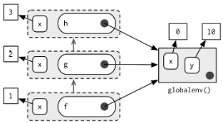
f()時的calling 環境中，所具有的參數為 (global) x =0, y = 10

g()時的calling 環境中，所具有的參數為 (f) x =1 , (global) y = 10

h()時的calling 環境中，所具有的參數為 (g) x =2 , (global) y = 10

將x設為3後，計算x+y=13，執行完成時f()、g()、h()各自所產生的封閉環境逐一瓦解，global 中的參樹依然沒有改變 x =0, y = 10

parent.frame：The parent.frame refers to the environment where the function was called from, not where it was defined.

Closures enclose the environment of the parent function and can access all its variables.

此時功能性(多層次)function設計可將參數劃分為兩種層級

parent level ：調控運作
child level：實際運作

範例中以一個 parent function (power()) 生成兩個 child functions (square() 和 cube())

power <- function(exponent) {
  function(x) {
    x ^ exponent
  }
}

square <- power(2)
cube <- power(3)
square(2)
## [1] 4
cube(2)
## [1] 8

square被設定為次方，cube則被設定為立方，但檢視兩者時會發現並無明顯不同

square
## function(x) {
##     x ^ exponent
##   }
## <environment: 0x3719630>


cube
## function(x) {
##     x ^ exponent
##   }
## <environment: 0x3870b58>

其實兩者的差異，是在於所擁有的environment包並不一致

square  :  <environment: 0x3719630>   
cube    :  <environment: 0x3870b58>

可用as.list(environment( )) 或是 pryr::unenclose() 查看environment包中的設定數值

as.list(environment(square))
## $exponent
## [1] 2
as.list(environment(cube))
## $exponent
## [1] 3

library(pryr)
unenclose(square)
## function (x) 
## {
##     x^2
## }
unenclose(cube)
## function (x) 
## {
##     x^3
## }

R中幾乎所有function都是Closure，Closure可獨立存取呼叫時所設立的資訊，而使其不會隨呼叫完成時一起消失 [有Java生成實體的感覺]

更多可參考 Advanced R by Hadley Wickham

[R] Lexical & Dynamic Scoping / Execution & Calling environments / Closures

猜你喜欢