4.2 数据集成

4.3数据变换

4.3.1 简单函数变换：

4.3.2 规范化（标准化）

4. 数据预处理

数据清洗、数据集成、数据交换、数据规约 à 提高信号质量。在整个建模过程中占比很长 60%~80%。

4.1数据清洗：

删除无关重复数据，平滑噪声，筛选掉无关数据，处理缺失值异常值

4.1.1 缺失值处理：删除缺失记录、补插、不处理

删除：最有效、但是局限性很大（通过减少历史数据来增加数据的完备性 à 浪费资源和隐藏的信息，可能影响客观性和准确性）

补插：

补插方法	描述
mean, media, most_freqently	均值，中位数，众数插补
固定值	将缺失属性值用固定值替换，如：外来打工人员的工资3000代替
最近邻插补	样本中最接近的样本的属性值插补
回归	根据已有数据和其他相关属性的数据建立模型回归预测
插值	利用已知点建立合适的插值函数，近似代替

拉格朗日插值法：

牛顿插值法：

与拉格朗日插值最终的结果相同，python中只提供了拉格朗日插值法；如果要使用牛顿插值法需要自己编写代码。

牛顿插值法：迭代阶差商公式

f(x1,x)=fx-f(x1)x-x1

f(x2,x1,x)= fx1,x-f(x2,x1)x-x2

f(x3,x2,x1,x)= fx2,x1,x-fx3,x2,x1x-x3

….

f(xn,xn-1,…,x2,x1,x)= fxn-1, ….. ,x2,x1,x-f(xn,…x3,x2,x1)x-xn

then:

f(x)=P(x)+Q(x)

P(x)=f(x1)+(x-x1)f(x2,x1)+(x-x1)(x-x2)f(x3,x2,x1)+….+(x-x1)(x-x2)….(x-x(n-1))f(x1,x2,x3,…,x(n-1))

Q(x)= (x-x1)(x-x2)….(x-xn)f(x1,x2,x3,…,xn,x))

代码：

# -*- coding: utf-8 -*-

"""

Created on Fri Feb 9 11:53:37 2018

@author: 康宁

"""

import pandas as pd

from scipy.interpolate import lagrange

import numpy as np

input_path='D:\迅雷下载\《Python数据分析与挖掘实战》\图书配套数据、代码\chapter3\demo\data\catering_sale.xls'

output_path='D:\迅雷下载\《Python数据分析与挖掘实战》\图书配套数据、代码\chapter3\demo\data\catering_sale_null.xls'

data=pd.read_excel(input_path)#,index_col=u'日期')

#data=pd.read_excel(input_path,index_col=u'日期')

data[u'销量'][(data[u'销量']>5000)|(data[u'销量']<400)]=None

##可以用query()和where() 实现筛选df.query('b == ["a", "b", "c"]'); df.query('[1, 2] not in c'); #isin(), not in s;

statistics_0=data.describe()

temp_notnull=data[data[u'销量'].notnull()]

#注意：在pandas里面，dataframe和series类型的数据 使用‘=’实在内存空间中重新开拓空间，与python本身的库不同

temp_isnull=data[data[u'销量'].isnull()]

n=3 #注意取n=5 时会产生过拟合，有些值会离奇的大，有些值离奇的小使用拉格朗日插值最大输入不能超过32个数

for i in list(temp_isnull.index):

x=pd.Series(list(range(i-n,i))+list(range(i+1,i+1+n)))

x=x[(x>=0)&(x<=len(data)) ] #此处需要使用布尔判断，所以转换为series类型

y=data.loc[x,u'销量']

f=lagrange(list(x),list(y))

‘’’ # Parameters

----------

x : array_like

`x` represents the x-coordinates of a set of datapoints.

w : array_like

`w` represents the y-coordinates of a set of datapoints, i.e. f(`x`).

‘’’

data.loc[i,u'销量']=f(i)

statistics_1=data.describe()

print(statistics_0,'\n',statistics_1)

print(data.loc[temp_isnull.index])

Help on property:

A primarily label-location based indexer, with integer position

fallback.

``.ix[]`` supports mixed integer and label based access. It is

primarily label based, but will fall back to integer positional

access unless the corresponding axis is of integer type.

``.ix`` is the most general indexer and will support any of the

inputs in ``.loc`` and ``.iloc``. ``.ix`` also supports floating

point label schemes. ``.ix`` is exceptionally useful when dealing

with mixed positional and label based hierachical indexes.

However, when an axis is integer based, ONLY label based access

and not positional access is supported. Thus, in such cases, it's

usually better to be explicit and use ``.iloc`` or ``.loc``.

See more at :ref:`Advanced Indexing <advanced>`.

help(pd.DataFrame.loc)

Help on property:

Purely label-location based indexer for selection by label.

``.loc[]`` is primarily label based, but may also be used with a

boolean array.

Allowed inputs are:

- A single label, e.g. ``5`` or ``'a'``, (note that ``5`` is

interpreted as a *label* of the index, and **never** as an

integer position along the index).

- A list or array of labels, e.g. ``['a', 'b', 'c']``.

- A slice object with labels, e.g. ``'a':'f'`` (note that contrary

to usual python slices, **both** the start and the stop are included!).

- A boolean array.

- A ``callable`` function with one argument (the calling Series, DataFrame

or Panel) and that returns valid output for indexing (one of the above)

``.loc`` will raise a ``KeyError`` when the items are not found.

See more at :ref:`Selection by Label <indexing.label>`

help(pd.DataFrame.iloc)

Help on property:

Purely integer-location based indexing for selection by position.

``.iloc[]`` is primarily integer position based (from ``0`` to

``length-1`` of the axis), but may also be used with a boolean

array.

Allowed inputs are:

- An integer, e.g. ``5``.

- A list or array of integers, e.g. ``[4, 3, 0]``.

- A slice object with ints, e.g. ``1:7``.

- A boolean array.

- A ``callable`` function with one argument (the calling Series, DataFrame

or Panel) and that returns valid output for indexing (one of the above)

``.iloc`` will raise ``IndexError`` if a requested indexer is

out-of-bounds, except *slice* indexers which allow out-of-bounds

indexing (this conforms with python/numpy *slice* semantics).

See more at :ref:`Selection by Position <indexing.integer>`

销量

count 195.000000

mean 2744.595385

std 424.739407

min 865.000000

25% 2460.600000

50% 2655.900000

75% 3023.200000

max 4065.200000

销量

count 201.000000

mean 2757.914262

std 436.629037

min 865.000000

25% 2468.300000

50% 2681.300000

75% 3033.100000

max 4162.340000

日期销量

0 2015-03-01 2681.300000

8 2015-02-21 4162.340000

14 2015-02-14 3658.435000

103 2014-11-08 3221.830780

110 2014-11-01 2919.119171

144 2014-09-27 2501.641656

D:/迅雷下载/《Python数据分析与挖掘实战》/图书配套数据、代码/chapter3/demo/code/temp.py:17: SettingWithCopyWarning:

A value is trying to be set on a copy of a slice from a DataFrame

See the caveats in the documentation: http://pandas.pydata.org/pandas-docs/stable/indexing.html#indexing-view-versus-copy

data[u'销量'][(data[u'销量']>5000)|(data[u'销量']<400)]=None

IX Indexer is Deprecated

Warning Starting in 0.20.0, the .ix indexer is deprecated, in favor of the more strict .iloc and .loc indexers.

.ix offers a lot of magic on the inference of what the user wants to do. To wit, .ix can decide to index positionally OR via labels depending on the data type of the index. This has caused quite a bit of user confusion over the years.

The recommended methods of indexing are:

.loc if you want to label index

.iloc if you want to positionally index.

In [97]: dfd = pd.DataFrame({'A': [1, 2, 3],

....: 'B': [4, 5, 6]},

....: index=list('abc'))

....:

In [98]: dfd

Out[98]:

A B

a 1 4

b 2 5

c 3 6

Previous Behavior, where you wish to get the 0th and the 2nd elements from the index in the ‘A’ column.

In [3]: dfd.ix[[0, 2], 'A']

Out[3]:

a 1

c 3

Name: A, dtype: int64

Using .loc. Here we will select the appropriate indexes from the index, then use label indexing.

In [99]: dfd.loc[dfd.index[[0, 2]], 'A']

Out[99]:

a 1

c 3

Name: A, dtype: int64

This can also be expressed using .iloc, by explicitly getting locations on the indexers, and using positional indexing to select things.

In [100]: dfd.iloc[[0, 2], dfd.columns.get_loc('A')]

Out[100]:

a 1

c 3

Name: A, dtype: int64

For getting multiple indexers, using .get_indexer

In [101]: dfd.iloc[[0, 2], dfd.columns.get_indexer(['A', 'B'])]

Out[101]:

A B

a 1 4

c 3 6

The most robust and consistent way of slicing ranges along arbitrary axes is described in the Selection by Position section detailing the .iloc method. For now, we explain the semantics of slicing using the [] operator.With Series, the syntax works exactly as with an ndarray, returning a slice of the values and the corresponding labels:

In [31]: s[:5]

Out[31]:

2000-01-01 0.469112

2000-01-02 1.212112

2000-01-03 -0.861849

2000-01-04 0.721555

2000-01-05 -0.424972

Freq: D, Name: A, dtype: float64

In [32]: s[::2]#正序步进为2输出

Out[32]:

2000-01-01 0.469112

2000-01-03 -0.861849

2000-01-05 -0.424972

2000-01-07 0.404705

Freq: 2D, Name: A, dtype: float64

In [33]: s[::-1]#逆序输出

Out[33]:

2000-01-08 -0.370647

2000-01-07 0.404705

2000-01-06 -0.673690

2000-01-05 -0.424972

2000-01-04 0.721555

2000-01-03 -0.861849

2000-01-02 1.212112

2000-01-01 0.469112

Freq: -1D, Name: A, dtype: float64

http://pandas.pydata.org/pandas-docs/stable/indexing.html#ix-indexer-is-deprecated

If you want to identify and remove duplicate rows in a DataFrame, there are two methods that will help: duplicated and drop_duplicates. Each takes as an argument the columns to use to identify duplicated rows.

D.duplicated() returns a boolean vector whose length is the number of rows, and which indicates whether a row is duplicated.

D.drop_duplicates() removes duplicate rows.

By default, the first observed row of a duplicate set is considered unique, but each method has a keep parameter to specify targets to be kept.

keep='first' (default): mark / drop duplicates except for the first occurrence.

keep='last': mark / drop duplicates except for the last occurrence.

keep=False: mark / drop all duplicates.

Set / Reset Index¶

Occasionally you will load or create a data set into a DataFrame and want to add an index after you’ve already done so. There are a couple of different ways.

Set an index¶

DataFrame has a set_index method which takes a column name (for a regular Index) or a list of column names (for a MultiIndex), to create a new, indexed DataFrame:

In [324]: data

Out[324]:

a b c d

0 bar one z 1.0

1 bar two y 2.0

2 foo one x 3.0

3 foo two w 4.0

In [325]: indexed1 = data.set_index('c')

In [326]: indexed1

Out[326]:

a b d

z bar one 1.0

y bar two 2.0

x foo one 3.0

w foo two 4.0

In [327]: indexed2 = data.set_index(['a', 'b'])

In [328]: indexed2

Out[328]:

c d

a b

bar one z 1.0

two y 2.0

foo one x 3.0

two w 4.0

The append keyword option allow you to keep the existing index and append the given columns to a MultiIndex:

In [329]: frame = data.set_index('c', drop=False)

In [330]: frame = frame.set_index(['a', 'b'], append=True)

In [331]: frame

Out[331]:

c d

c a b

z bar one z 1.0

y bar two y 2.0

x foo one x 3.0

w foo two w 4.0

Other options in set_index allow you not drop the index columns or to add the index in-place (without creating a new object):

In [332]: data.set_index('c', drop=False)

Out[332]:

a b c d

z bar one z 1.0

y bar two y 2.0

x foo one x 3.0

w foo two w 4.0

In [333]: data.set_index(['a', 'b'], inplace=True)

In [334]: data

Out[334]:

c d

a b

bar one z 1.0

two y 2.0

foo one x 3.0

two w 4.0

Reset the index¶

As a convenience, there is a new function on DataFrame called reset_index which transfers the index values into the DataFrame’s columns and sets a simple integer index. This is the inverse operation to set_index

In [335]: data

Out[335]:

c d

a b

bar one z 1.0

two y 2.0

foo one x 3.0

two w 4.0

In [336]: data.reset_index()

Out[336]:

a b c d

0 bar one z 1.0

1 bar two y 2.0

2 foo one x 3.0

3 foo two w 4.0

The output is more similar to a SQL table or a record array. The names for the columns derived from the index are the ones stored in the names attribute.

You can use the level keyword to remove only a portion of the index:

In [337]: frame

Out[337]:

c d

c a b

z bar one z 1.0

y bar two y 2.0

x foo one x 3.0

w foo two w 4.0

In [338]: frame.reset_index(level=1)

Out[338]:

a c d

c b

z one bar z 1.0

y two bar y 2.0

x one foo x 3.0

w two foo w 4.0

reset_index takes an optional parameter drop which if true simply discards the index, instead of putting index values in the DataFrame’s columns.

Note

The reset_index method used to be called delevel which is now deprecated.

4.1.2 异常值处理

删除
视为缺失值	按照缺失值处理办法进行修正
平均值修正	取前后两个观测值的平均值修正
不处理	直接在异常数据基础上建模

4.2 数据集成

多个数据源合并 à 一个数据库中 à 表达形式不一样，不匹配，属性冗余 à 转换、提炼、集成

实体识别：同名异意，异名同义，单位不统一

冗余识别：同一属性多次出现，同一属性命名不同 à 避免数据不一致 à 提高挖掘速度与质量（参见3.2.6 相关性分析 person相关系数，spearman相关系数，判定系数）

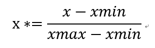
4.3数据变换

对数据规范化处理，便于程序和挖掘分析。

4.3.1 简单函数变换：

（开方，平方，取对数，差分）：

（非正态分布-> 正态分布）

（非平稳序列->平稳序列（时间序列分析，有时通过简单的差分和对数运算即可完成））

4.3.2 规范化（标准化）

通过比例缩放，消除同一属性不同量纲、不同属性之间数值差异比较大的情况

1. 最小最大标准化（离差标准化）:

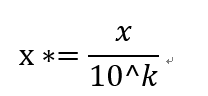
(注意：若是遇到属性值超出【min，max】范围会出错，需要重新确定max和min)

2. 零-均值标准化（标准差标准化）：

3. 小数定标标准化：

移动属性值的小数位数讲属性值映射到 [-1,1]之间

# -*- coding: utf-8 -*-

"""

Created on Fri Feb 9 11:53:37 2018

@author: 康宁

"""

import pandas as pd

path='D:\迅雷下载\《Python数据分析与挖掘实战》\图书配套数据、代码\chapter4\demo\data\normalization_data.xls'

data=pd.read_excel(path)

data_max=data.max()

data_min=data.min()

data_mean=data.mean()

data_std=data.std()

data_normal_min_max=(data-data_min)/(data_max-data_min)

data_mornal_mean_std=(data-data_mean)/(data_std)

#data.abs().max()

#np.log10(data.abs().max())

k=np.ceil(np.log10(data.abs().max()))

data_10=data*10**(-k)

4.3.3 连续属性离散化

分类算法（ID3,Apiroi）要求数据是分类属性形式 à 要求将连续属性转换为分类属性

任务：

1. 确定分类数，分类点；

（等宽法：对离群值敏感，各个区间分布不均匀，甚至极少，损坏决策模型；

等频法：避免等宽法缺点；

聚类分析法）

2. 将连续属性映射到分类属性分类区间不同符号数值代表不同区间上的连续属性值

#----------------------------------------------------------------------------------------------------------

import pandas as pd

import numpy as np

k=5 #组数

path='D:\迅雷下载\《Python数据分析与挖掘实战》\图书配套数据、代码\chapter4\demo\data\discretization_data.xls'

data=pd.read_excel(path)

data=data[u'肝气郁结证型系数']

#等宽分布

d1=pd.cut(data,bins=k,labels=range(k)) #pd.cut(实现连续值到离散区间之间的切分，labels默认为None,此时返回的标签是分组的区间，retbins 设置是否返回分割点)

#等频分布

w=np.linspace(0,1,k+1)

l=data.describe(percentiles=w)[4:].drop(['max'])

if k%2==1:

l=l.drop(['50%'])

#利用D.describe()计算分位数实现等频分布，percentiles为分位数列表

l[0]=l[0]*(1-1e-2)

l[-1]=l[-1]*(1+1e-2) #扩大区间，防止边界值的标签为None

d_efreq=pd.cut(data,bins=l,labels=range(k),retbins=False)

from sklearn.cluster import KMeans

if __name__=='__main__':

kmodel=KMeans(n_clusters=k,n_jobs=1,random_state=123)

kmodel.fit(data.reshape(-1,1))

cent=pd.DataFrame(kmodel.cluster_centers_,columns=['position']).sort_values(by='position',axis=0)

#输出聚类中心，并且排序（默认是随机序的）

d_kmeans=kmodel.labels_

d_kmeans_boundary=list(pd.rolling_mean(cent,window=2 )['position'])+[data.max()]

d_kmeans_boundary[0]=data.reshape(-1,1).min()

import matplotlib.pyplot as plt

import matplotlib as mpl

plt.rcParams['font.sans-serif'] = ['SimHei'] #用来正常显示中文标签

plt.rcParams['axes.unicode_minus'] = False #用来正常显示负号

def cluster_plot(d,k):

plt.figure()

for i in range(k):

plt.plot(data[d==i],i*np.ones(data[d==i].count()),'o')

plt.show()

return plt

cluster_plot(d1,k)

cluster_plot(d_efreq,k)

cluster_plot(d_kmeans,k)

4.3.4 属性构造

利用已有属性构造新的属性 --> 加入到现有属性集

import pandas as pd

path='D:\迅雷下载\《Python数据分析与挖掘实战》\图书配套数据、代码\chapter4\demo\data\electricity_data.xls'

output_path='D:\迅雷下载\《Python数据分析与挖掘实战》\图书配套数据、代码\chapter4\demo\data\electricity_outputfile.xls'

d=pd.read_excel(path)

d[u'线损率']=(d[u'供入电量']-d[u'供出电量'])/d[u'供入电量']

d.to_excel(output_path)

供入电量	供出电量
986	912
1208	1083
1108	975
1082	934
1285	1102

	供入电量	供出电量	线损率
0	986	912	0.075051
1	1208	1083	0.103477
2	1108	975	0.120036
3	1082	934	0.136784
4	1285	1102	0.142412

4.3.5小波变换

新型数据分析工具：信号处理、图像处理、语音处理、模式识别、量子物理

特点:多分辨率（在信号时域和频域均有表征信号局部特征的能力）

伸缩和平移变换 多出都聚焦分析 –> 非平稳信号的时域分析手段

将信号分解表达不同层次，不同频带信息的数据序列 --> 就是 小波系数

方法：

基于小波变换的多尺度空间能量分布提取：	各尺度空间的平滑信号和细节信号能够提供原始信号的时频局域信息，特别是不同频段上信号的构成信息。把不同尺度上的能量信号求解出来，就可以将这些能量尺度顺序排列，形成特征向量供识别使用
多尺度空间的模极大值提取；	利用小波变换的信号局域化分析能力，求解小波变换的模极大值特性来检测信号的局域奇异性，将小波变换的模极大值参数s，平移参数t，及其幅值作为目标的特征量
基于小波变换的特征提取；	利用小波分解，将时域随机信号序列映射为尺度域各子空间内的随机系数序列，按小波包分解得到最佳子空间内随机系数序列的不确定程度最低，将最佳子空间的熵值以及最佳子空间的完整二叉树中的位置参数作为特征量，可以用于目标识别
基于是适应性的小波网络的特征提取	基于适应性小波神经网络的特征提取方法可以把信号通过分析小波拟合表示，进行特征提取

小波基函数

小波变换

基于小波变换的多尺度空间能量分布特征提取方法

path='D:\迅雷下载\《Python数据分析与挖掘实战》\图书配套数据、代码\chapter4\demo\data\leleccum.mat'

from scipy.io import loadmat

import pywt

mat=loadmat(path)

signal=mat['leleccum']

coeffs=pywt.wavedec(signal,'bior3.7', level = 5)

小波分析这里没有看懂，后面需要仔细补足这里的理论知识

4.4数据规约

产生更小的保持源数据完整性的新数据集 --> 后续的挖掘&分析更高效

降低无效的 &错误数据对建模的影响，提高建模的准确性
少量更具代表性的数据：计算成本à 减少计算量、减小建模时间、降低存储成本

4.4.1属性规约

属性合并&删除不相关属性(同时确保新属性集的概率分布尽可能和原分布相同) à 减少数据维数 à 降低计算成本

方法：

属性规约方法	描述
合并属性	直接删除不相关属性	旧属性合并为新属性
逐步向前选择		每次从原始属性集中选出最佳的属性放到新的属性集中，直至满足阈值或者无法继续选择新属性为止
逐步向后删除		与逐步向前恰好相反，逐步删除
决策树归纳		决策树归纳，没有在决策树上的属性, 认为无关，删除
主成分分析PCA	构造原始数据的正交变换，新空间的基底去除了原始空间基底下属性之间的相关性，使用少量的新属性（主成分PCA）就可以解释原始的大部分属性

主成分分析PCA：

分析流程：

求协方差矩阵
求特征值和特征向量λ1>λ2>λ3>λ4> … > λn & β1、β2、β3 … βn

βi=[β11, β21, β31, … βni]T

构造新的属性值Zi= [X1 X2 X3 … Xn]* βi；（优先选取特征值大的特征向量，这样构造出的新属性方差更大，是我们想要的结果）

from sklearn.decomposition import PCA

#PCA 参数说明：

n_components 意义：PCA分析中要保留的主成分or特征个数；如果赋值为’string’类型，则自动选择特征个数，使之满足所要求的方差百分比。
copy：bool，默认True 表示运行算法时是否将原始数据复制一份；若为False，运行算法时训练数据值会改变；
whiten：bool类型，默认False，使每个特征具有相同的方差

# -*- coding: utf-8 -*-

"""

Created on Mon Feb 12 12:33:34 2018

@author: 康宁

"""

import pandas as pd

path='D:\迅雷下载\《Python数据分析与挖掘实战》\图书配套数据、代码\chapter4\demo\data\principal_component.xls'

outpath='D:\迅雷下载\《Python数据分析与挖掘实战》\图书配套数据、代码\chapter4\demo\data\principal_component_l_data.xls'

data=pd.read_excel(path)

from sklearn.decomposition import PCA

pca=PCA()

pca.fit(data)

pca.components_

pca.n_components

pca.explained_variance_ratio_

pca3=PCA(3)

pca3.fit(data)

l_data=pca3.transform(data)

pca3.components_

pca3.explained_variance_ratio_

l_h=pca3.inverse_transform(l_data)

pd.DataFrame(l_data).to_excel(outpath)

pca_whiten=PCA(3,whiten=True)

pca_whiten.fit(data)

whiten_data=pca_whiten.transform(data)

4.4.2数值规约

替代的、较小的数据减少数据量

有参数：线性回归，多元回归，对数线性模型（近似离散属性的集中的多维概率分布）

无参数：存放实际数据，如：直方图、聚类（将对象归为簇，用数据的簇替换实际的数据）、抽样（有放回抽样，无放回抽样，聚类抽样（总共M个簇，抽出S个簇出来），分层抽样）

4.5 python主要数据预处理函数

name	function	module
interpolate	一维或者高维数据插值	Scipy
unique	去除数据中的重复元素	Pandas/Numpy
isnull/notnull	判断是否空值/非空值	Pandas
PCA	对指标变量矩阵进行主成分分析	Scikit-Learn
random	生成随机矩阵	Numpy

from Scipy.interpolate import lagrange

from Scipy.interpolate import *

f=lagrange(x,y)

f(new_x)

np.unique(D); #代表1-D list, array, Series;

D.unique(); #D是Pandas的Series对象

isnull/notnull

D.isnull()/D.notnull()

D[D.isnull()]/D[D.notnull()]

np.random.rand(k,m,n) #生成（k,m,n）的随机矩阵，数值均匀分布（0，1）

np.random.randn(k,m,n) #生成（k,m,n）的随机矩阵，数值服从标准正太分布（0，1）

PCA

from sklearn.decomposition import PCA

model=PCA()

model.fit()

modle.n_components_

model.explained_variance_ratio_

《数据分析与挖掘实战》总结及代码练习---chap4 数据预处理

4. 数据预处理

4.1数据清洗：

4.1.1 缺失值处理：删除缺失记录、补插、不处理

4.1.2 异常值处理

4.2 数据集成

4.3数据变换

4.3.1 简单函数变换：

4.3.2 规范化（标准化）

4.3.3 连续属性离散化

4.3.4 属性构造

4.3.5小波变换

4.4数据规约

4.4.1属性规约

4.4.2数值规约

4.5 python主要数据预处理函数

猜你喜欢