搭配词(collocation)
广义而言,搭配词(collocation)是指两个或多个词一招语言习惯性结合在一起表示某种特殊意义的词汇。搭配词在不同的研究领域上又不同的解读,尚未有一致性的定义。大概的意思就是词语的习惯搭配了,就是学英语时老师一直拿来搪塞我们的那种『习惯搭配』。比如sit in traffic,表示堵车或者在通勤上花费了非常多时间的意思,那么sit_traffic就是一个搭配词。其中sit称为base word,traffic称为collocate. 所以collocations = base word + collocate.
前面的例子中介词in去哪里了呢?研究搭配词时通常只研究base word和collocate两个单词,可以记为 ,比如sit和traffic的collocation表示为(sit, traffic),中间的单词都省略掉。这样的表示类似bigram的形式,称为skip bigram,即跳过(skip)中间的一些词,只取首尾两个词记为bigram的形式。普通的bigram也是skip bigram的一种。
虽然skip bigram跳过了中间的词,但不意味着这部分信息丢失了。skip bigram有个距离属性,表示skip bigram中首尾两个词中间相差多少个词。两个相连的词构成的skip bigram距离是1,比如sit in traffic的(sit, in)的距离为1,所以没有距离为0的bigram!但是有距离是负数的bigram,比如(in, sit)的距离为-1,表示sit应该在前面。对于英语,这个距离一般取5和-5.
类似地,sit in traffic的所有skip bigram(包含普通bigram在内)有如下,括号中的数字表示距离。
- (sit, in, 1)
- (in, traffic, 1)
- (in, sit, -1)
- (traffic, in, -1)
- (sit, traffic, 2)
- (traffic, sit, -2)
搭配词研究的意义在于有些词合在一起可能符合语法,但平常几乎不会用,或者合在一起没有什么意义,那么从语料库中找出常用的搭配词就可以用于英文学习或句子改错。比如你非要说stand in traffic,语法上看起来没有错误,但(stand, traffic, 1)在语料库中出现的次数很低,因为没有人这么说。
Smadja算法
算法思想
搭配词选取通常从语料库中用统计的方法选出一些候选词,然后判断哪些搭配词是合理的搭配词。常用的统计方法又互信息,log likelihood ratio (LLR),t检验,chi-square检验等。另外一种方法是Smadja于1993年提出的基于ngram距离的语法关系搭配词提取方法(Syntactic relation by distanced ngram analysis)。基本思想是:
- 计算任意两个单词在距离d时一起出现的次数,即距离为d的skip bigram的个数
对于英文最大距离取5,最小距离取-5. 比如(play, role)在距离-4~4之间出现的次数如下表所示。
| 距离 | (play, role) count |
|---|---|
| -4 | 81230 |
| -3 | 161358 |
| -2 | 920270 |
| -1 | 255149 |
| 1 | 27584 |
| 2 | 1428845 |
| 3 | 3452577 |
| 4 | 325548 |
- 选取出现次数最高的skip bigram作为最终的collocation,此时它们的距离是
.
比如上表中可以看到当play和role的距离为3是他们出现的次数是最多的,此时(play, role, 3)就是最终的搭配词,例如play an important role.
Smadaj算法有两个基本假设:
- 搭配词出现的频率远高于非搭配词,即(base word, collocate)出现的频率高于其它组合
- 搭配词出现的次数在距离上的分布有峰值
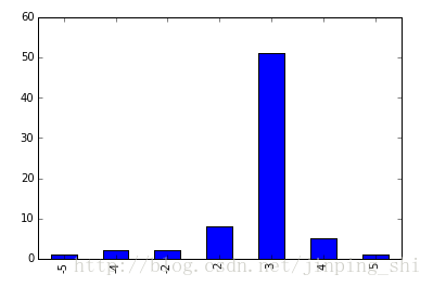
如下图是(play, role)在距离-5~5之间的频率分布,可以看到在距离为3时出现峰值。
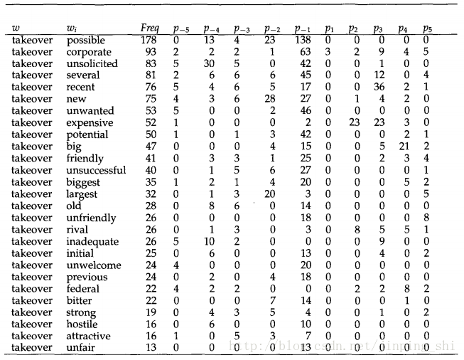
为了应用Smadaj算法,我们需要计算出任意两个单词的skip bigram出现的次数以及它在每个距离上出现的次数。下图是Smadaj论文中的图。图中base word是takeover,显示的是takeover与所有搭配词的频率分布。
得到上表后Smadja提出了三个条件来筛选合理的搭配词。一些符号表示如下。
记某个base word
与它的搭配词
的频率是
,即上表中
那一列。记某个base word的平均频率为
,即上表中
一列的平均值,表示base word takeover的平均频率。记
为搭配词
在距离
上出现的次数,
为搭配词
在所有距离上出现次数的平均值,即:
Smadja算法中判断搭配词
是否合理的三个条件是:
其中 , . , 和 是需要自己定义的阈值。Smadja给出的经验值是 , , .
这三个条件直接,简单,粗暴。解释如下。
中的 实际上是将 标准化,计算 的 -score. 可以筛掉在整个语料库中出现频率不高的搭配词。
中的 就是搭配词在各个距离上频率分布的方差。如果某个搭配词 的 很小,表示它在各距离上的频率分布十分均匀,表示它可能并不是一个合理的搭配词。因为合理的搭配词一般在某个距离上出现的次数很多,在其它距离上出现的次数很少,导致 会很大。
和 可以筛选出上表中那些搭配词是合理的, 可以筛选出这些合理的搭配词的距离。 在搭配词在距离上的分布基础上,将距均值 倍标准差的项目筛选出来,实际上跟 一样,也是利用 -score来筛选。
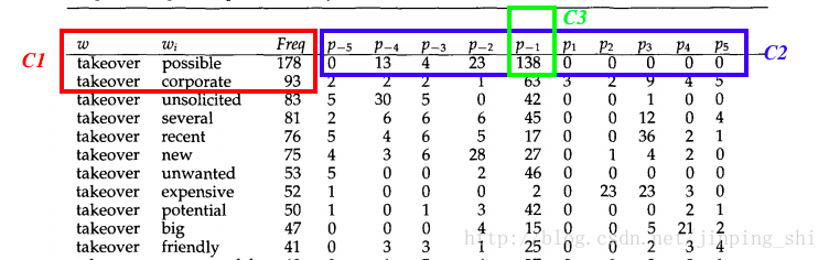
三个条件的作用如下图所示。 可以选出 和 ,接着 从这两个候选词中选出 ,最后 告诉我们 搭配的距离是-1,即这个搭配词的合理用法可能是possible + some word + takeover.
虽然Smadja的方法提出迄今好二十多年了,但是仍然很有用。
算法实现
以下是Smadja算法的Python实现。算法本身不难,难的是如何将代码写得Pythonic.
求n-gram
如果距离取5,那么就需要求出所有的bigram,trigram,4-gram和5-gram的组合,然后计算出skip bigram. 下面是求这些n-gram的代码。
定义一个defaultdict类型的变量ngram_counts来存放n-gram以及它在每个距离上出现的次数。ngram_counts的key是n-gram中的n,value是一个Counter. Counter也相当于dict,它的key是以tuple形式保存的n-gram,value是这个n-gram在语料库中出现的次数。
from nltk.tokenize import  wordpunct_tokenize
from nltk.corpus import stopwords
from collections import defaultdict, Counter

k0            = 1
k1            = 1
U0            = 10
max_distance  = 5

eng_stopwords = set(stopwords.words('english'))
eng_symbols   = '{}"\'()[].,:;+!?-*/&|<>=~$'

def ngram_is_valid(ngram):
    first, last = ngram[0], ngram[-1]
    if first in eng_stopwords or last in eng_stopwords: return False
    if any( num in first or num in last for num in '0123456789'): return False
    if any( eng_symbol in word for word in ngram for eng_symbol in eng_symbols): return False
    return True

# 求句子的n-gram
def to_ngrams( unigrams, length):
    return zip(*[unigrams[i:] for i in range(length)])

ngram_counts = defaultdict(Counter)
with open('citeseerx_descriptions_sents.txt.50000') as text_file:
    for index,line in enumerate(text_file):
        words = wordpunct_tokenize(line)
        for n in range(2, max_distance + 2):
            ngram_counts[n].update(filter(ngram_is_valid, to_ngrams(words, n)))
比如要查看5-gram,上述代码输出的结果如下:
>> ngram_counts[5]
Counter({('In', 'this', 'paper', 'we', 'present'): 179, ('In', 'this', 'paper', 'we', 'describe'): 73, ('In', 'this', 'paper', 'we', 'propose'): 66, ('This', 'paper', 'presents', 'a', 'new'): 39})
求skip bigram
求出n-gram后需要将n-gram转化为skip bigram. 即求出skip bigram在各个距离上的频率分布。
skip bigram的形式是
,同样定义一个三层的defaultdict类型变量skip_bigram_info来保存skip bigram结果。skip_bigram_info的key是base word,value是一个dict,value的key是collocate,对应的value是一个Counter,Counter的key是距离,value是这个搭配词在对应距离上出现的次数。
如何求skip bigram?
可以发现,比如一个5-gram ('In', 'this', 'paper', 'we', 'present')的次数是179,那么('In', 'present', 4)出现的次数一定是179(最后一个数字代表skip bigram的距离)。所以只要取每个n-gram首尾的两个词组成skip bigram,就可以得到这个skip bigram在距离
上的次数。
skip_bigram_info = defaultdict(lambda: defaultdict(Counter))
for dist in range(2, max_distance + 2):
    for ngram, count in ngram_counts[dist].items():
        skip_bigram_info[ngram[0]][ngram[-1]] += Counter({dist-1: count})
        skip_bigram_info[ngram[-1]][ngram[0]] += Counter({1-dist: count}) # 求负向距离,单词对调,距离求相反数即可
我们想看看base word为play的搭配词,可以输入skip_bigram_info['play'],得到如下结果:
defaultdict(collections.Counter,
            {'Acquaintances': Counter({-1: 1}),
             'Agent': Counter({-2: 1}),
             'C': Counter({-1: 1}),
             'Domain': Counter({-3: 1}),
             'Elimination': Counter({-2: 1}),
             'Groups': Counter({-3: 1}),
             'In': Counter({-5: 1}),
             'Interconnect': Counter({-2: 1}),
             'Interest': Counter({-4: 1, -2: 2}))
查看(play, role)在各个距离上的分布,输入skip_bigram_info['play']['role']:得到
Counter({-5: 1, -4: 2, -2: 2, 2: 8, 3: 51, 4: 5, 5: 1})计算筛选条件
根据
,
,
计算一些统计量
。这些统计量都按照tuple的形式存在dict类型的变量skip_bigram_abc中。以(play, role)为例,存储的形式如下:
skip_bigram_abc[play, 'avg_freq']
skip_bigram_abc[play, 'avg_freq']
skip_bigram_abc[('play','role','spread')]
skip_bigram_abc[('play','role','freq')]
计算各统计量代码如下。
skip_bigram_abc = defaultdict(lambda: 0)
for word, vals in skip_bigram_info.items():
    count = []
    for coll, val in vals.items():
        c = val.values()
        c_bar = sum(c) / (2*max_distance)
        skip_bigram_abc[(word, coll, 'freq')] = sum(c)
        skip_bigram_abc[(word, coll, 'spread')] = (sum([x**2 for x in c]) - 2*c_bar*sum(c) + 2*max_distance*c_bar**2) / (2 * max_distance)
        count.append(sum(c))
    skip_bigram_abc[(word, 'avg_freq')] = np.mean(count)
    skip_bigram_abc[(word, 'dev')] = np.std(count)
根据上述计算的统计量,再计算符合条件的skip gram,同样保存在一个dict类型的变量cc中,存储格式如下:
# cc = [('base word', 'collocate', 'distance', 'strength', 'spread', 'peak', 'p'), ...]筛选符合条件的skip bigram代码如下:
def skip_bigram_filter(skip_bigram_info, skip_bigram_abc):
    cc = []
    for word, vals in skip_bigram_info.items():
        f = skip_bigram_abc[(word, 'avg_freq')]
        for coll, val in vals.items():
            if skip_bigram_abc[(word, 'dev')]-0 < 1E-6:
                strength = 0
            else:
                strength = (skip_bigram_abc[(word, coll, 'freq')] - f) / skip_bigram_abc[(word, 'dev')]
            if strength < k0:
                continue
            spread = skip_bigram_abc[(word, coll, 'spread')]
            if spread < U0:
                continue
            c_bar = sum(val.values()) / (2*max_distance)
            peak = c_bar + k1 * math.sqrt(spread)
            for dist, count in val.items():
                if count >= peak:
                    cc.append((word, coll, dist, strength, spread, peak, count))
    return cc

cc = skip_bigram_filter(skip_bigram_info, skip_bigram_abc)
结果展示
将cc转成pandas的DataFrame格式,比较好操作。
import pandas
collocations_df = pandas.DataFrame(cc,
columns = ['base word', 'collocate', 'distance', 'strength', 'spread', 'peak', 'p'])
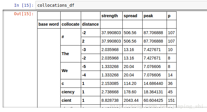
collocations_df = collocations_df.set_index(['base word', 'collocate', 'distance']).sort_index()pandas的DataFrame结构可以在Jupyter Notebook显示成表格,效果如下图所示。
完整的代码可以参考Smadja Algorithm.
完整的代码中还包括如何筛选特定POS tagging的搭配词的代码,比如筛选VB-NN关系的搭配词(动词-名词形式)。有兴趣的可以参考。
Reference
- Frank Smadja, Retrieving Collocations from Texts: Xtract, Computational Linguistics, Volume 19, 1993.
- 基於統計方法之中文搭配詞自動擷取