opencv 直方图

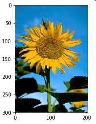
A = cv2.imread(‘E:/python/sunflower.png’,0)
hist=cv2.calcHist([A],[0],None,[256],[0,256])

第一个参数为原图像
第二个参数为通道数，gray[0],bgr[0],[1],[2]
第三个参数掩模，统计某一部分图像直方图，此时需要掩模图像，若全图则None
第四个为bin直方条数目
第五个参数为像素值范围
hist返回值为256*1数组

hist,bins=np.histogram(img.ravel(),256,[0,256])
ravel可以将图像转为一维数组
hist=np.bincount(img.ravel(),minlength=256)
可以计算一维直方图，计算速度快

绘制直方图

plt.hist(A.ravel(),256,[0,256])
plt.show

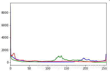
A = cv2.imread('E:/python/sunflower.png')
color=('b','g','r')
for i,col in enumerate(color):
    hist=cv2.calcHist([A],[i],None,[256],[0,256])
    plt.plot(hist,color=col)
    plt.xlim([0,256])

plt.show

在这里插入图片描述

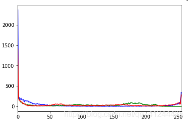
带掩模

import cv2
import numpy as np
import matplotlib.pyplot as plt
 
A = cv2.imread('E:/python/sunflower.png')
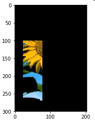
mask=np.zeros(A.shape[:2],np.uint8)
mask[100:270 ,23:78]=255
masked_img=cv2.bitwise_and(A,A,mask=mask)
color=('b','g','r')
for i,col in enumerate(color):
    hist=cv2.calcHist([A],[i],mask,[256],[0,256])
    plt.plot(hist,color=col)
    plt.xlim([0,256])

plt.show

在这里插入图片描述
直方图均衡化

import cv2
import numpy as np
import matplotlib.pyplot as plt
 
A = cv2.imread('E:/python/sunflower.png',0)
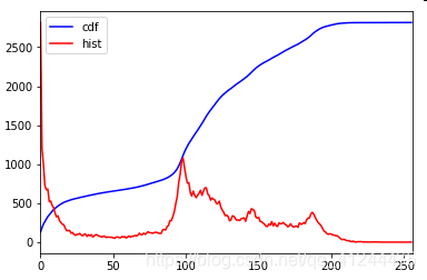
hist,bins=np.histogram(A.flatten(),256,[0,256])
#计算积分图
cdf=hist.cumsum()
cdf_normalized=cdf*hist.max()/cdf.max()
plt.plot(cdf_normalized,color='b')
plt.plot(hist,color='r')
plt.xlim([0,256])
plt.legend(('cdf','hist'),loc='upper left')
plt.show()
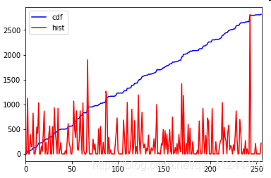
#直方图均衡化
cdf_m=np.ma.masked_equal(cdf,0)
cdf_m=(cdf_m-cdf_m.min()*255/(cdf_m.max()-cdf_m.min()))
cdf=np.ma.filled(cdf_m,0).astype('uint8')
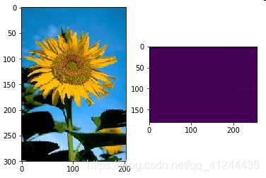
img2=cdf[A]

plt.subplot(121),plt.imshow(A)
plt.subplot(122),plt.imshow(img2)

在这里插入图片描述

equ=cv2.equalizeHist(imgray)
res=np.hstack((A,equ))#此处是将原图与均衡化图组成一个数组

#局部均衡
clahe=cv2.createCLAHE(clipLimit=2.0,tileGridSize=(8,8))
cl=clahe.apply(A)
plt.imshow(cl,‘gray’)

https://docs.opencv.org/3.1.0/d5/daf/tutorial_py_histogram_equalization.html

2D直方图

#2Dhist
hsv=cv2.cvtColor(A,cv2.COLOR_BGR2HSV)
hist=cv2.calcHist([hsv],[0,1],None,[180,256],[0,180,0,256])
A=A[:,:,::-1]
plt.subplot(121),plt.imshow(A)
plt.subplot(122),plt.imshow(hist,interpolation='nearest')
plt.imshow

在这里插入图片描述

hist,xbins,ybins=np.histogram2d(hsv[:,:,0].ravel,hsv[:,:,1].ravel,[180,256],[[0,180],[0,256]])

反向投影：图像分割或者寻找感兴趣区域反向投影

import cv2
import numpy as np
import matplotlib.pyplot as plt
 
A = cv2.imread('E:/python/fxc.png')
target = cv2.imread('E:/python/fx.png')
hsv=cv2.cvtColor(A,cv2.COLOR_BGR2HSV)
roi=cv2.cvtColor(target,cv2.COLOR_BGR2HSV)
hist=cv2.calcHist([hsv],[0,1],None,[180,256],[0,180,0,256])
cv2.normalize(hist,hist,0,255,cv2.NORM_MINMAX)#归一化
dst=cv2.calcBackProject([roi],[0,1],hist,[0,180,0,256],1)
disc=cv2.getStructuringElement(cv2.MORPH_ELLIPSE,(5,5))
dst=cv2.filter2D(dst,-1,disc)
ret,thresh=cv2.threshold(dst,127,255,0)
thresh=cv2.merge((thresh,thresh,thresh))
res=cv2.bitwise_and(target,thresh)
res=np.hstack((A,target,thresh,res))
cv2.imshow('1',thresh)
k = cv2.waitKey(0) 
if k == ord('s'):        
    cv2.destroyAllWindows()

猜你喜欢