
Kp1,kp2都是list类型,两幅图都是500个特征点。这和ORB论文中的数据是一样的。4.4章节
Matches也是list类型,找到325个匹配对。
AKAZE文章中提到一个指标:MS(matching score)=# Correct Matches/# Features,
如果overlap area error 小于40%并且经矩阵变换后两个对应像素距离小于2.5个像素,就说明是correct match。这里的overlap area error没有搞懂,应该在Mikolajczyk的A comparison of affine region dectors中找到答案。
还没搞清楚的还有:代码中的matches指的应该是correspondence,因为ORB论文中有一句perform brute-force matching to find the best correspondence.代码中使用的正是BFMatcher。但是文章接下来给出的曲线图是The results are given in terms of the percentage of correct matches, against the angle of rotation.
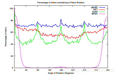
the percentage of correctmatches应该等效于图上的纵坐标percentage of Inliers。那么percentage of和Inliers指的都应该是经过RANSAC提纯之后的匹配对。ORB文章中没有提到提纯,即剔除误匹配对的过程。
img3 = drawMatches(img1, kp1, img2, kp2, matches[:50])#找到50个匹配对
在绘制匹配对的时候,代码直接对匹配器中的50个进行连线。但是看到其他代码中还有一个排序的过程:
matches=sorted(matches,key=lambda x:x.distance)首先,Python中有两种排序方法,一种是sort,一种是Sorted。
L.sort(cmp=None, key=None, reverse=False) -- stable sort *IN PLACE*
Sort默认升序排序。要想颠倒排序,可将默认的False改为True。In place说明sort是就地排序,直接改变原来list
sorted(iterable, cmp=None, key=None, reverse=False) --> new sorted list
sorted会新建一个list,用来存放排序之后的数据
cmp:用于比较的函数,比较什么由key决定,有默认值,迭代集合中的一项;
key:用列表元素的某个属性和函数进行作为关键字,有默认值,迭代集合中的一项;
cmp和key可以使用lambda表达式。
可以理解为是cmp按照key的比较结果排序,而key直接按照参数排序。因为列表中的元素很可能是元组。简单来说,lambda返回冒号之后的值。下面两种方法是等价的
Sorting cmp:
>>>L = [('b',2),('a',1),('c',3),('d',4)]
>>>print sorted(L,cmp=lambda x,y:cmp(x[1],y[1]))
[('a', 1), ('b', 2), ('c', 3), ('d', 4)]
>>>L = [('b',2),('a',1),('c',3),('d',4)]
>>>print sorted(L, key=lambda x:x[1]))
[('a', 1), ('b', 2), ('c', 3), ('d', 4)]
Lamdba是匿名函数,有函数体,没有函数名,常用作回调函数的值。函数对象能维护状态,但语法开销大,而函数指针语法开销小,却没法保存范围内的状态。lambda函数结合了两者的优点。
Lambda还经常和Reduce函数放在一起使用。Reduce函数其实是一个具有递归作用的二元函数,对集合中的前两个执行函数,得到的结果再与第三个元素做运算,以此类推。
Reduce(lambda x,y:x*y,range(1,n+1)) #n的阶乘
sum=reduce(lambda x,y:x+y,(1,2,3,4,5,6,7)) #1+2+…+7
bf = cv2.BFMatcher(cv2.NORM_HAMMING, crossCheck=True)#暴力匹配,True判断交叉验证先使用cv.BFMatcher创造一个BfMatcher的对象。第一个参数normType,规定了匹配时使用的距离准则,默认是cv2.NORM_L2欧式距离,适用于SIFT、SURF等。对于二进制字符串构成的描述子如ORB、BRIEF、BRISK等,使用cv2.NORM_HAMMING汉明距离。汉明距离可以通过异或快速求解,这也是算法加速的原因。最后,If ORB is using WTA_K == 3 or 4, cv2.NORM_HAMMING2 should be used.
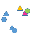
第二个参数crossCheck,是布尔型参数,默认为false。如果改为True,就开启了交叉验证,我理解的就是双向匹配,只有双向匹配成功的匹配对才被返回。数学上讲,有两个集合A和B,对于集合A中的i,在B中找到的最近点是j,如果对于j,在A中搜索,找到的最近点也是i,那么他们就验证成功。如下图,黄色的三角形在圆的集合中找到的最近点是绿色的圆。但是对于绿圆,最近的点的粉色的三角,即交叉验证失败。就像是找对象,必须男女双方互相看对眼才能牵手成功。当然,我们可以直接比较两个距离的大小,距离小于某个阈值认为匹配正确,SIFT则提出了最近邻和次近邻的比值与阈值比较。
It provides consistant result, and is a good alternative to ratio test proposed by D.Lowe in SIFT paper.手册上说这种交叉验证的方法可以是SIFT文章所提的最近邻比率法的一个很好的代替。
在创建BfMatcher的对象之后,有两种匹配方法,BFMatcher.match() and BFMatcher.knnMatch()。第一种返回的是最好的匹配对,第二种是返回k个最好的匹配对,k的取值由用户定义。两种匹配对对应的连线方法cv2.drawMatches()和cv2.drawMatchesKnn。这里再记录一下drawmatches的参数
void cv::drawMatches 	( 	InputArray  	img1,
		const std::vector< KeyPoint > &  	keypoints1,
		InputArray  	img2,
		const std::vector< KeyPoint > &  	keypoints2,
		const std::vector< DMatch > &  	matches1to2,
		InputOutputArray  	outImg,
		const Scalar &  	matchColor = Scalar::all(-1),
		const Scalar &  	singlePointColor = Scalar::all(-1),
		const std::vector< char > &  	matchesMask = std::vector< char >(),
		int  	flags = DrawMatchesFlags::DEFAULT
	)
前四个参数分别是两幅图像和各自的特征点,matches1to2表明匹配的方向是从图1到图2,keypoints1[i] has a corresponding point in keypoints2[matches[i]] .
outImg是输出的图像。
matchColor决定了连线和特征点的颜色,如果matchColor==Scalar::all(-1) ,颜色随机生成。
singlePointColor决定了没有对应匹配对的孤立特征点的颜色
matchesMask决定哪些匹配对被画出,如果掩膜为空,则所有匹配对都被画出
flags是所画特征点的标志位, DEFAULT = 0,默认会画出所有特征点
BFMatcher.knnMatch()主要用于配合SIFT文章中的最近邻比率法使用。当最近的距离小于次近邻的0.75时(这个阈值的取值很重要,0.75出自于OpenCV手册,Lowe的论文中选取0.7),认为是正确匹配对。手册中是以SIFT算法为例展示了knn的用法,实际在ORB中也可以使用Knn和近邻比率法进行配对。
比率法在寻找最近距离的过程中综合考虑了次近邻,这样,只有当点很明显是最接近的情况下才会认为配对。对于一些疑似是对应点,但疑似情况差不多的点就不再认为是匹配点,即便他们与当前特征点的绝对距离都很近。
由KNN算法还可以引入kd数的构建和BBF算法,更快地在搜索空间中寻找k个近邻点。OpenCV中也集成了一个快速搜索最近邻的库FLANN(Fast Library for Approximate Nearest Neighbors),可以在特征点的描述子的维度高,特征点数目大的情况下依然快速找到最近邻点。写到这里可以注意到,当KNN中的K取1时就是最近邻。所以之前的BFMatcher中的BFMatcher.match() and BFMatcher.knnMatch()都可以通过FLANN实现。
基于FLANN的检测器主要有两个字典类型的参数,index_params和search_params。
#index_params与所选取的特征点检测算法有关

index_params = dict(algorithm = FLANN_INDEX_KDTREE, trees = 5)#kd树,对应SIFT、SURF

index_params= dict(algorithm = FLANN_INDEX_LSH, table_number = 6, key_size = 12, # 20

multi_probe_level = 1) #2 #LSH局部敏感哈希,对应ORB
第二个参数search_params决定了迭代的次数。It specifies the number of times the trees in the index should be recursively traversed.迭代次数越多,准确度越高,但是耗时当然也越长。
Index参数和search参数定义好之后就可以创建搜索器并进行匹配了。
# FLANN parameters
16 FLANN_INDEX_KDTREE = 0
17 index_params = dict(algorithm = FLANN_INDEX_KDTREE, trees = 5)
18 search_params = dict(checks=50)   # or pass empty dictionary
19
20 flann = cv2.FlannBasedMatcher(index_params,search_params)
21  #根据描述子进行k=2的knn搜索
22 matches = flann.knnMatch(des1,des2,k=2)
23
24 # Need to draw only good matches, so create a mask
#xrange是一个生成器。这里对matches进行标记,初始化为0.注意每一个match有最近和次近邻两个匹配点
25 matchesMask = [[0,0] for i in xrange(len(matches))]
26
27 # ratio test as per Lowe's paper
#对于最近邻m和次近邻n,如果最近距离小于次近邻的0.7,那么就将m标记成1,从而得到0,1组成的掩膜
28 for i,(m,n) in enumerate(matches):
29     if m.distance < 0.7*n.distance:
30         matchesMask[i]=[1,0]
31
32 draw_params = dict(matchColor = (0,255,0),
33                    singlePointColor = (255,0,0),
34                    matchesMask = matchesMask,
35                    flags = 0)#利用掩膜,只画出最好的匹配的对
36
37 img3 = cv2.drawMatchesKnn(img1,kp1,img2,kp2,matches,None,**draw_params)
Matches是list类型的,里面存放了DMatch类型的匹配对,每个DMatch有4个成员变量:distance(float)、imgIdx(int)、queryIdx(int)、trainIdx(int),表示了匹配对中特征点的距离,索引等信息。query是要匹配的描述子,train是被匹配的描述子

这是k=2时KNN的输出结果,对于每一个query,会匹配前两个最近邻的特征点。List中的元素是list,每一个list元素由两个DMatch构成。
经过最近邻比率法提纯后:
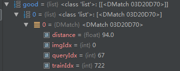
可以看到,直到query的第67个点才达成第一个正确匹配。
利用经过最近邻比率法匹配得到的匹配对,得到新的描述子,再通过新的描述子寻找单应矩阵,寻找单应矩阵的过程中又可以使用RANSAC等方法提纯。
遇到的问题是函数cv2.findHomography的第一第二个参数要求是array或者scalar类型的,srcPoints Coordinates of the points in the original plane, a matrix of the type CV_32FC2. or vector\<Point2f\> .。
python中的list是python的内置数据类型,list中的数据类不必相同的,而array的中的类型必须全部相同,the type of objects stored in them is constrained,The type is specified at object creation time by using a type code, which is a single character.。在list中的数据类型保存的是数据的存放的地址,简单的说就是指针,并非数据,这样保存一个list就太麻烦了,例如list1=[1,2,3,'a']需要4个指针和四个数据,增加了存储和消耗cpu。
des1是ndarray类型的,包含383个特征点,每个特征点的描述子的维度是61(AKAZE),所以是一个383x61大小的矩阵。
忙活了半天把初始描述子中属于good的部分提取出来并转化成ndarray格式,却发现cv2.findHomography的前两个参数是特征点,而不是特征点的描述子,并且OpenCV又已经在链接5中给出了示例。
这是最终的图像配准代码:
#!/usr/bin/env.python
#coding=utf-8
## coding=gbk 支持中文注释
import numpy as np
import cv2
import math
import logging
orig_image=cv2.imread("beaver.png",0)
skewed_image=cv2.imread("beaver_xform.png",0)

cv2.imshow("graf1",orig_image)
cv2.imshow("graf2",skewed_image)


#定义函数
def mydrawMatches(orig_image, kp1, skewed_image, kp2, matches):
    rows1=orig_image.shape[0]#height(rows) of image
    cols1=orig_image.shape[1]#width(colums) of image
    #shape[2]#the pixels value is made up of three primary colors
    rows2=skewed_image.shape[0]
    cols2=skewed_image.shape[1]

#初始化输出的新图像,将两幅实验图像拼接在一起,便于画出特征点匹配对
    out=np.zeros((max([rows1,rows2]),cols1+cols2,3),dtype='uint8')

    out[:rows1,:cols1] = np.dstack([orig_image, orig_image, orig_image])#Python切片特性,初始化out中orig_image,skewed_image的部分
    out[:rows2,cols1:] = np.dstack([skewed_image, skewed_image, skewed_image])#dstack,对array的depth方向加深

    for mat in matches:
        orig_image_idx=mat.queryIdx
        skewed_image_idx=mat.trainIdx

        (x1,y1)=kp1[orig_image_idx].pt
        (x2,y2)=kp2[skewed_image_idx].pt

        cv2.circle(out,(int(x1),int(y1)),4,(255,255,0),1)#蓝绿色点,半径是4
        cv2.circle(out, (int(x2) + cols1, int(y2)), 4, (0, 255, 255), 1)#绿加红得黄色点
        cv2.line(out, (int(x1), int(y1)), (int(x2) + cols1, int(y2)), (255, 0, 0), 1)#蓝色连线

    return out

# 检测器。ORB AKAZE可以,KAZE需要将BFMatcher中汉明距离换成cv2.NORM_L2
detector = cv2.AKAZE_create()

#kp1 = detector.detect(orig_image, None)
#kp2 = detector.detect(skewed_image, None)
#kp1, des1 = detector.compute(orig_image, kp1)#计算出描述子
#kp2, des2 = detector.compute(skewed_image, kp2)

#也可以一步直接同时得到特征点和描述子
# find the keypoints and descriptors with ORB

kp1, des1 = detector.detectAndCompute(orig_image, None)
kp2, des2 = detector.detectAndCompute(skewed_image, None)

bf = cv2.BFMatcher(cv2.NORM_HAMMING, crossCheck=True)#暴力匹配,True判断交叉验证
matches = bf.match(des1, des2)#利用匹配器得到相近程度
matches=sorted(matches,key=lambda x:x.distance)#按照描述子之间的距离进行排序
img3=cv2.drawMatches(orig_image, kp1, skewed_image, kp2, matches[:50],None,(255, 0, 0),flags=2)#找到50个匹配对

 # Apply ratio test
bf = cv2.BFMatcher(cv2.NORM_HAMMING, crossCheck=False)#为了得到最近邻和次近邻,这里交叉验证要设置为false
matches = bf.knnMatch(des1,des2, k=2)
good = []
#lenofgood=0
for m, n in matches:
    if m.distance < 0.75 * n.distance:

        good.append([m])#good.append(m)
        #lenofgood=lenofgood+1

#matches2 = sorted(good, key=lambda x: x.distance)  # 按照描述子之间的距离进行排序
 # cv2.drawMatchesKnn expects list of lists as matches.
#img4 = cv2.drawMatches(orig_image, kp1, skewed_image, kp2, matches2[:50],None, flags=2)
#img4 = cv2.drawMatchesKnn(orig_image, kp1, skewed_image, kp2, good[:50],None, flags=2)
img4 = cv2.drawMatchesKnn(orig_image, kp1, skewed_image, kp2, good,None, flags=2)
lenofgood=len(good)#good长度为24

des1fromgood=np.ones((lenofgood,61),dtype=np.uint8)
#des2fromgood=[]
des2fromgood=np.ones((lenofgood,61),dtype=np.uint8)
for num in range(0,24):
    for i in good:
        for j in i:
        #good是list组成的list,每个子list中是DMatch
            des1fromgood[num]=des1[j.queryIdx]#将good中的特征点对应的描述子形成新的描述子
            #des2fromgood.append(des2[j.trainIdx])
            des2fromgood[num] = des2[j.trainIdx]

cv2.imwrite("AKAZETest.jpg", img3)
cv2.imshow('AKAZETest', img3)
cv2.imwrite("AKAZETestRatio.jpg", img4)
cv2.imshow('AKAZETestRatio', img4)

#H,mask=cv2.findHomography(des1fromgood,des2fromgood,cv2.RANSAC,5.0)#,None,None,None,None,None)
good = []
for m, n in matches:
    if m.distance < 0.7 * n.distance:
        good.append(m)
MIN_MATCH_COUNT = 10
if len(good) > MIN_MATCH_COUNT:
    src_pts = np.float32([kp1[m.queryIdx].pt for m in good
                                  ]).reshape(-1, 1, 2)
    dst_pts = np.float32([kp2[m.trainIdx].pt for m in good
                                  ]).reshape(-1, 1, 2)

    M, mask = cv2.findHomography(src_pts, dst_pts, cv2.RANSAC, 5.0)
    ss = M[0, 1]
    sc = M[0, 0]
    scaleRecovered = math.sqrt(ss * ss + sc * sc)
    thetaRecovered = math.atan2(ss, sc) * 180 / math.pi
    #logging打印出通过矩阵计算出的尺度缩放因子和旋转因子
    LOG_FORMAT = "%(asctime)s - %(levelname)s - %(message)s"
    DATE_FORMAT = "%m/%d/%Y %H:%M:%S %p"

    logging.basicConfig(filename='my.log', level=logging.DEBUG, format=LOG_FORMAT, datefmt=DATE_FORMAT)
    #配置之后将log文件保存到本地
    logging.info("MAP: Calculated scale difference: %.2f, "
                  "Calculated rotation difference: %.2f" %
                  (scaleRecovered, thetaRecovered))

    # deskew image
    im_out = cv2.warpPerspective(skewed_image, np.linalg.inv(M),
                                 (orig_image.shape[1], orig_image.shape[0]))
    result=cv2.warpPerspective(orig_image,M,(skewed_image.shape[1],skewed_image.shape[0]))
    #注意warpPerspective与warpAffine的区别,不能互换
#img_warp=cv2.perspectiveTransform(orig_image,M)#,img_warp)
#c.shape[1] 为第一维的长度,c.shape[0] 为第二维的长度。
cv2.imshow("fan透视变换",im_out)
cv2.imshow("透视变换",result)
cv2.waitKey(0)
reference:
- Lambda:https://blog.csdn.net/zcy19941015/article/details/47053799
- OpCVtutorial:https://docs.opencv.org/3.1.0/dc/dc3/tutorial_py_matcher.html
- 切片特性https://www.jianshu.com/p/5083f8d75439
- List指针https://blog.csdn.net/liyaohhh/article/details/51055147
- https://www.programcreek.com/python/example/70413/cv2.RANSAC