[CS294-112] model-based RL

版权声明：Copyright reserved to Hazekiah Wang ([email protected]) https://blog.csdn.net/u010909964/article/details/85329751

Content

1 Control and Planning

• 1.1 Stochastic Optimization
• 1.2 MTCS
• 1.3 LQR
• 1.4 iLQR/DDP

2 Model-Based RL

• 2.1 version 0.5
• 2.2 version 1.0
• 2.3 MPC
• 2.4 PILCO
• 2.5 model-based v.s. model-free
• 2.6 what model to choose

3 Local Models

• 3.1 motivation
• 3.2 used in what scenarios
• 3.3 how to fit local models

4 policy learning with a learned model

• 4.1 short-coming of PILCO
• 4.2 GPS
• 4.3 Imitating with DAgger
• 4.4 DAgger v.s. GPS
• 4.5 Dyna

5 How to choose methods

• 5.1 sample efficiency rank
• 5.2 a rough road map for RL methods

1. Control and Planning

Open-loop Trajectory optimization methods
assumptions: a (learned) dynamics model in hand
objective: find the optimal action sequence that maximizes the expected return of the trajectories given that action sequence under the known dynamics model.

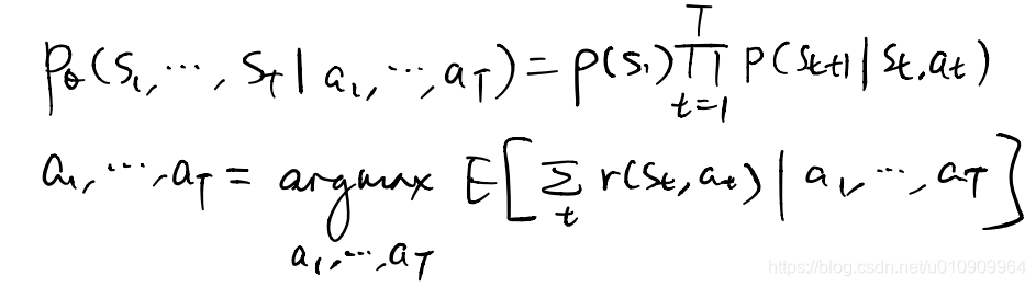
inputs: a dynamics model, a cost function (to minimize)

side note open-loop versus closed-loop control
open-loop = no-feedback system
closed-loop = feedback system
feedback means process output is required for next decision.

1.1 stochastic optimization

1.1.1 random shooting
generate random action sequences from an arbitrary distribution, and take the sequence among them that yields the lowest cost as the final solution.

weakness in high-dim action space, there are low odds to sample the optimal actions. (the curse of dimensionality)

1.1.2 CEM: Cross-Entropy Methods

loop {
	1. generate samples (action sequences) from a parameterized distribution.  
	2. evaluate costs and pick the lowest k samples  
	3. fit the distribution to the k samples
}

intuition use a parameterized distribution that adapt to the lower cost action space iteratively.

1.1.3 CMA-ES
like CEM with momentum

1.2 Monte Carlo Tree Search with Upper Confidence Bounds for Trees

MCTS
Given: a root node, a TreePolicy, a DefaultPolicy

do {
	1. get to a leaf node according to the TreePolicy
	2. rollout the node according to the DefaultPolicy until a terminating state.
	3. compute the reward of the rollout trajectory, update the statistics along the route from current leaf node to the root node
} until some criterion met.

DefaultPolicy
Given: a node (state)

1. sample an action uniformly from the allowed action space of the state
2. return the next state (inferred under the known dynamics)

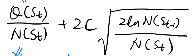
TreePolicy: UCT (Upper Confidence Bounds for Trees) algorithm
Given: the root node

1. do {
	1. choose the best child node of the current node according to the UCT function
	2. set the current node the best child node.
} until the current node is expandable.

2. randomly choose an action from the allowed action space of the current node.
3. get to the next state under the known dynamics.
4. expand the current node with a new node of this state, return this child node.

The statistics of each node includes the total reward and number of visits of the subtree with itself as the root.

As to how we define the goodness of a child, we use the UCT fuction. The UCT function balances against exploration and exploitation, intuitively prefers to expand those nodes that are less visited than their siblings with high average returns.

side note this is straight-forward for the deterministic dynamics, for the stochastic case, some reparameterization tricks are required

Case Study
Deep Learning for Real-Time Atari Game Play Using Offline Monte-Carlo Tree Search Planning
combines DAgger with MCTS as such

loop {
	1. train a policy on state-action pairs D
	2. run the policy to obtain unseen states {o_j}
	3. label the states with actions suggested by MCTS to forge state-action pairs D_u
	4. aggregate D with D_u
}

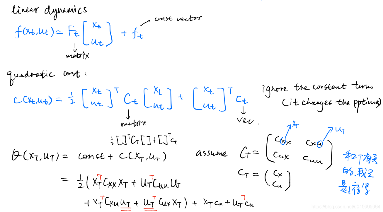
1.3 Linear Quadratic Regulator (LQR)

given: a linear dynamics function, a quadratic cost (Q) function

objective: find the action sequence that minimizes the cost function under the dynamics.

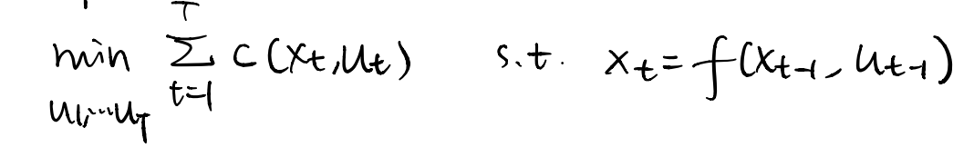
and with the substitution of the dynamics constraint, we turn it to an unconstrained optimization problem.

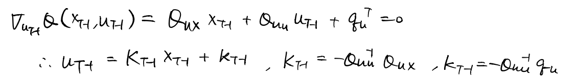
At time step t, we first optimizes Q to get the optimal action.

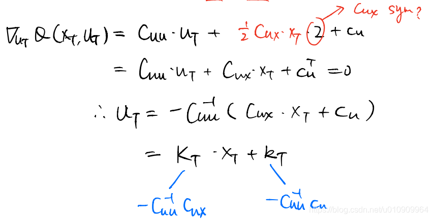
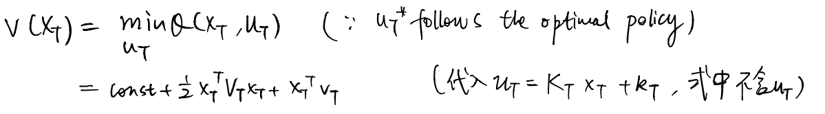
And we compute the optimum, which is the value at this state.

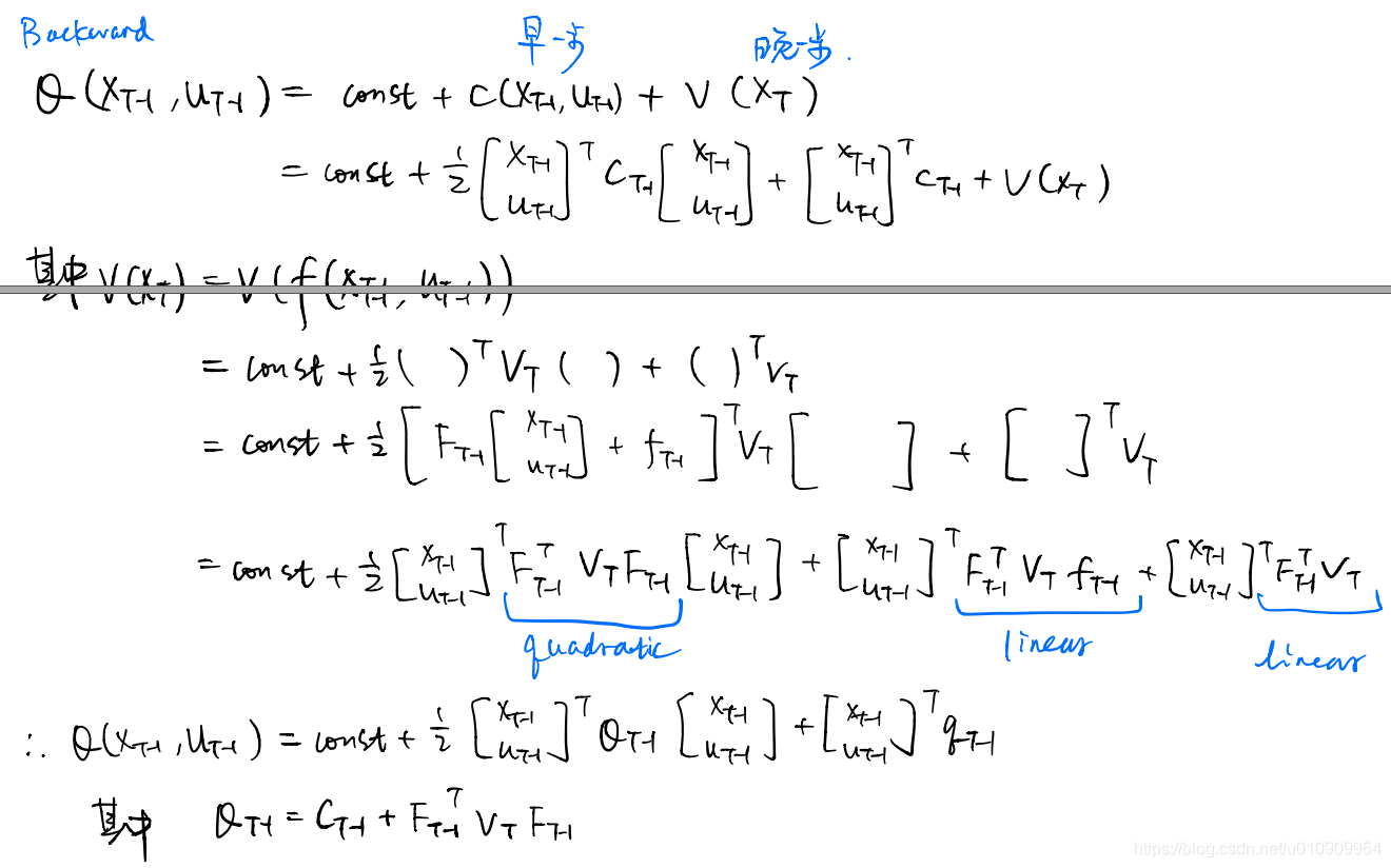
For the last time step t-1, we clean the Q-function via Bellman Backup, into the form of a quadratic.

Again we solve for the optimal action at time t-1.

==> 1.3.1 The Deterministic case
logics

loop {
	1. At time t we can find the optimal action w.r.t the  Q-function. (The action is a linear function of the state)
	2. Since this action optimizes the cost function, it also optimizes the Q-function. Substituting the a_t = K_t*s_t+k_t into the Q-function, we obtain the optimal value at time t, with the only variable s_t. Now the value-function is a quadratic function of s_t.
	3. At time t-1, based on Bellman Backup, the Q-function equals the current step cost plus the next step value-function. We obtained the time t value-function w.r.t s_t, and now we substitute s_t with the dynamics function to get rid of s_t. Now we obtain the Q_function at time t-1 dependent on only variable s_{t-1} and a_{t-1}.
}

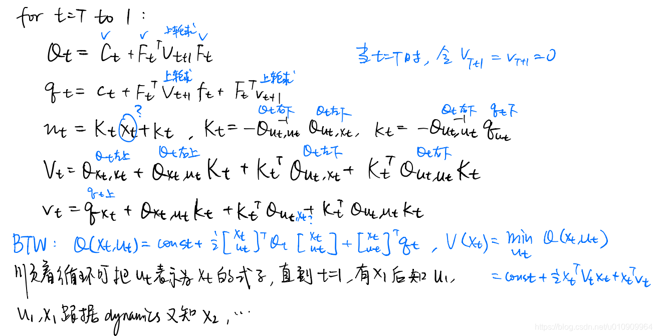
To summarize, this is a process backpropagating through time where we iteratively compute 1) the optimal action ( $a_t = f(s_t)$), 2) the value function ( $v = g(s_t)$), and 3) the last step Q-function ( $Q(s_{t-1},a_{t-1})$). What we get after this process is an optimal action sequence, each dependent on their corresponding inferred state, i.e. $a_t = f(s_t)$.

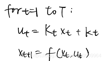
Next we do some forward recursion stuff:

t = 0, s_0 is known
loop {
	1. given s_t, compute a_t
	2. compute s_{t+1} based on the dynamics function
	3. t = t+1
} until t==T.

This is simple because we know the first state and the relationship of $a_t$ and $s_t$ at each time step, and this forms a recursion under the inference of the dynamics function.

After that we get the optimal action sequence.

==> 1.3.2 The Stochastic Case
In this case, the distribution of the dynamics is represented by a Gaussian with its mean linear w.r.t the inputs $a_t$ and $s_t$, and some constant variance matrix $\sigma_t$, also called linear-Gaussian.

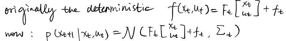
This is said to be solved by the same algorithm as the deterministic case.

side note shooting methods versus collocation methods
There are two formulations for trajectory optimization:

1. optimizes for the trajectory (state and action sequence), formulating the problem as a constrained optimization. The constraint is the dynamics and the objective is the expected return over state and action sequences.
2. optimizes only for the action sequence, formulating the problem as an unconstrained optimization by substituting the dynamics function into the objective function (to replace the states).

The first approach is called collocation and the second shooting. Shooting methods are figurative in their name. The optimal action sequence only depends on the state preceding it, which is true for any part of this action sequence. If there is error in any intermediate expected state, the true optimal action sequence will diverge from the current erroneous one and shoot in another way.

However, the collocation methods do not act in this way. They are like feedback system, only part of the trajectory will be infected by an intermediate erroneous state.

1.4 iLQR or DDP

Normally a system is not a linear one, the idea here is to approximate it locally and iterate to converge to an optimality like the Newton’s method.

How to approximate the dynamics and the cost (Q) function locally?
– Taylor Expansion at some point.

Then we manage to incorporate this into LQR.

initialize the sequences a and s.
do {
	1. recast the approximated linear dynamics at current a and s
	2. recast the approximated quadratic cost at current a and s
	3. run LQR backward pass on delta_a and delta_s (delta incurred by the Taylor Expansion)
	4. run LQR forward pass, with the approximated optimal action solution and the real dynamics.
	5. update a and s with the approximated solution
} until convergence.

This is called iterative LQR.

To move a bit towards the Newton’s methods, we can approximate the dynamics with second order expansion. The derived methods is called Differential Dynamic Programming.

2 Model-Based RL

2.1 version 0.5

loop {
	1. run a based policy to collect transitions D.
	2. fit a dynamics model to D.
}

After the dynamics model completes learning, use some control and planning methods with the learned model to give actions.

weakness distribution mismatch
The base policy forges a state distribution while the planner constructs another state distribution, and the two may not be a same distribution.

This matters because the planner wouldn’t give the optimal action if the model makes false prediction, since the planner’s decisions are based on the model’s predictions.

solution DAgger

2.2 version 1.0

run the base policy to obtain transitions D.
loop {
	1. fit the model to D.
	2. run the planner with the learned model, obtain some action sequences.
	3. interact with the environment to obtain the resulting transitions D_u.
	4. aggregate D with D_u.
}

benefits this is bridging the gap of distributions.
weakness The Compounding Errors
If the planner is an open-loop one, the errors incurred by the dynamics will be accumulated. Each of the planner’s decision is based on the model’s prediction. Upon the first small errors, the planner gives sub-optimal action, leading to a sub-optimal state. If such state still involves errors in the model’s prediction, based on that, the planner would gives sub-sub-optimal action. This is why errors are accumulated.

solution Replan right after the unexpected predictions.
Intuitively, we further ensure that the prediction of the planner’s potential outcome state is accurate.

2.3 version 1.5 (MPC: Model Predictive Control)

run a base policy to obtain transitions D.
loop {
	1. fit a model to D.
	2. loop {
		1. run the planner with current model, obtain an action sequence
		2. pick the first action to execute, interact with the environment, obtain a transition.
		3. aggregate D with this transition
		4. set current state (according to the interaction)
	}
}

benefits

1. get away with weaker planner.
   this is because, only the first action really matters and a powerful planner for the whole trajectory is no more necessary. For example, a random shooting planner can work well with MPC.
2. reduce the horizon.
   since only the first action matters, It is natural to turn to shorter plan which is easier.

side note The replan horizon can be set multi-steps.
This is kinda tradeoff of the replan cost and the compounding errors.

2.4 version 2.0 (PILCO)

1. run a base policy to obtain transitions D.
2. loop {
	1. fit a model to D
	2. generate some trajectories based on current policy.
	3. optimizes the parameterized policy with the expected return objective.
	4. run the learned policy to obtain transitions D_u
	5. aggregate D with D_u
}

Note that the mentioned objective is exactly the unconstrained optimization objective mentioned in trajectory optimization.
weakness
Computing gradients of the unconstrained objective involves the issues of vanishing gradient and exploding gradient, because there will be too long a chain of the dynamics function if the horizon is large.

side note
the stochastic case requires the application of reparameterization tricks.

Case Study
Learning to Control a Low-Cost Manipulator using Data-Efficient Reinforcement Learning

1. run a base policy to obtain transitions D.
2. loop {
	1. fit Gaussian Processes to D
	2. generate some trajectories based on current policy.
	3. optimizes the parameterized policy with the expected return objective.
	4. run the learned policy to obtain transitions D_u
	5. aggregate D with D_u
}

The interesting stuff lies in computing gradients.
Under stochastic case, if $p(s)$ is a Gaussian and we know $p(s'|s,a)$, $p(s')$ is not a Gaussian but has some closed-form analytic representation. They perform moment matching to approximates it with a Gaussian.
With a selected reward function, the gradients presents some convenient form to compute.

2.5 model-based versus model-free

Inference of model-free at test time is fast because do not need planning (esp. MPC)

Simulation cost is alleviated with model-based.

2.6 what kind of model to use

Gaussian Processes: efficient with small amount of low-dim data, but assumes smooth dynamics.
Neural Nets: expressive with large amount of data, but can easily overfit in low data regimes.
mixture models: deal with low-dim state space.

3 Local model

3.1 motivation

A global model needs to be accurate anywhere in the state space, and often does not.

If not, the planner using this global model tends to exploit thoses positive errors, i.e., the planner tends to seek out where the global model leads to high rewards, which might well involve the error of the model’s positive expectation of states.

solution Estimate a dynamics only locally around the state distribution the current policy might yield, and ensure this local model as accurate as possible.

3.2 what are the scenarios for local models

When the policy does not need the whole dynamics, i.e., the policy only exploits partial information from the dynamics.

e.g. 端水杯

3.3 fitting local models

If we follow the previous idea of fitting a local model to current policy, the algorithm is directly as follows:

initialize a policy (controller)
loop {
	1. collect data: run current policy and interact with the environment to obtain transitions.
	2. fit the local model to the data.
	3. improve the policy based on the learned model.
} until convergence

=======
side note policy and controller
Both of them refers to a process given states suggests optimal actions. Policy often is used in the context of RL, while controller the control theory.

=======
Here is one of the instantiations.

1. how to improve policy
This is straight-forward if we recall the previous iLQR. In fact, we mentioned that, in each iteration we uses the current trajectory to approximates the dynamics, which appears identical to local models we refer to here.

Assume we use iLQR, we need to approximate the dynamics with a linear function and the cost a quadratic, and the optimal action solution is linear to its corresponding state. Let’s rule out these one by one:

1. a linear dynamics
   We can assume the local model fitted in step 2 is a linear one. That is, we are exactly fitting the partial derivatives of the dynamics w.r.t $a_t$ and $s_t$. This is equivalent to doing first-order Taylor Expansion for the dynamics.

   Often the dynamics is a stochastic one, we can formulate a linear-Gaussian, i.e., a Gaussian with linear mean dynamics and constant variance. Note that under the stochastic case, iLQR still solves the problem.
   

2. a quadratic cost function
   Normally we want to maximize the expected return via the Q-function, we can approximate it with second-order Taylor Expansion.

   But there is more to discuss about.

3. the controller
   The solution, the optimal action, given by iLQR, is in the linear form of its dependent variable, the state. However there is more to discuss about.

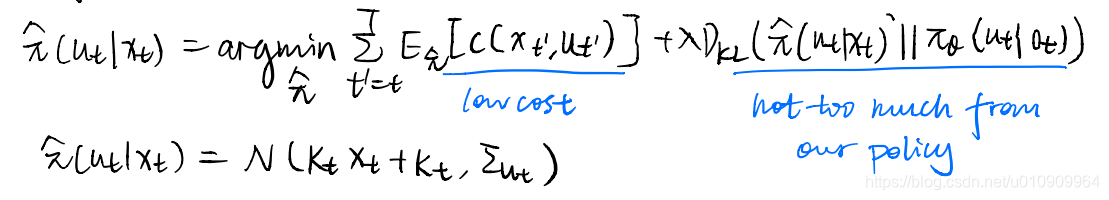
2. What controller to execute
The core issue here is that a deterministic controller is not proper. The explanation given by Sergey Levine is that the local model needs the data to be diverse to fit.

The resulting formulation for the controller is again a linear-Gaussian, with the optimal action as its mean. Then another question comes: how do we choose the variance matrix?

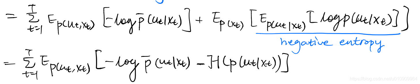
In other words, when do we need the actions to be diffuse and when gathered? When an actions matters (in the sense that the Q-function fluctuate if the action alters), we need it to be gathered, otherwise diffuse with high variance. It follows that we choose the inverse of the second derivative of Q w.r.t the action, which represents the curvation of surface Q-a at some state.

We can prove that, given a linear-Gaussian dynamics, a quadratic cost, the solution given by iLQR serves as the maximum entropy solution.

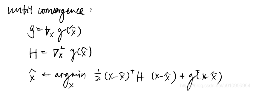
3. trust region
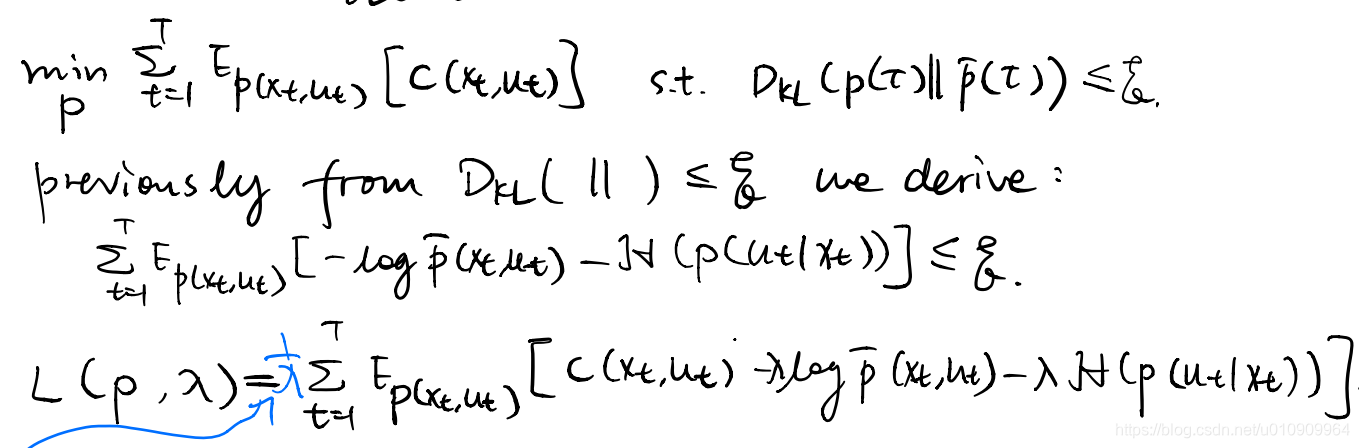
we approximate the dynamics linearly in local spots around the controller’s trjectories, meaning our local model only accurate in such places. Recall iLQR subjects to the constraint of the linear dynamics which is locally accurate, so we have to further constrain that the updated controller yields optimal trajectory in near local regions, so that the optimal solution is not too vulnerable to the approximation error.

Formally we constration the trajectory distribution before and after the controller update are close to each other. Specifically we can use the KL divergence as the measure of distribution distance. Then we derive something:



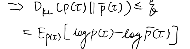
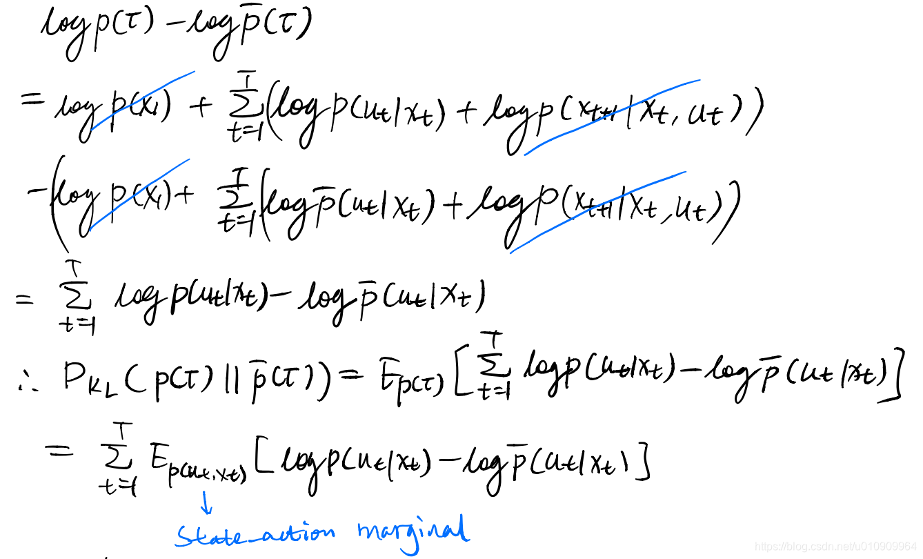
This serves an extra constraint for our trajectory optimization in step 3.

4. adaptation of iLQR
Now the problem transforms into a constrained problem. Note that the cost here equivalent to the objective function of iLQR, i.e., the expected return with the substitution of the dynamics. We solve this with Dual Gradient Descent.


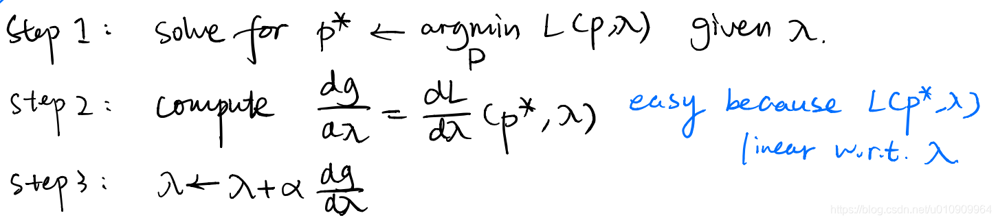
How can we make it through step 1? Recall that the linear-Gaussian controller solution given by iLQR solves for this objective, which is similar to ours. Simply we can do a recast of the cost to merge into the standard iLQR.

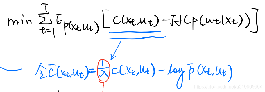
This cost function also provides some intuition: $\lambda$ controls the weight of the distribution distance, which is small initially, leading to loose bound. With the increase of $\lambda$, the importance of Q decreases by a factor of $\lambda$, in turn stressing more on the distribution distance bound.

Put these together

initialize a linear-Gaussian controller
loop {
	1. collect data: run the current controller and interact with the environment to obtain transitions.
	2. fit the linear-Gaussian dynamics to the data
	3. improve the policy: iLQR with DGD
	loop {
		1. recast the quadratic cost, given the learned linear-Gaussian dynamics, run iLQR to solve for the mean action.
		2. forges the controller with the mean action and the inverse of second derivative of Q
		3. compute gradients for lambda
		4. update lambda
	} until convergence
} until convergence

4 Learn a policy while learning a model

Potential benefits are: 1) no need for replan, 2) can do closed-loop control and 3) better generalization.

4.1 short-coming of direct backprop into the policy

We mentioned this approach as model-based version 2.0. This approach suffers from numerical instability similar to that of the recurrent nets. Intuitively speaking, our objective, the expected return, is the sum over a trajectory, and the earlier action influences more on the objective. As a result, the gradient of the objective w.r.t. earlier actions are large while the latter are small.

The latter actions have small gradients because they are computed by the chain rule, i.e., the same jacobian matrix has been multiplied by the times as the horizon, leading to potential vanishing gradient or exploding gradient, identical to BPTT.

4.2 Guided Policy Search

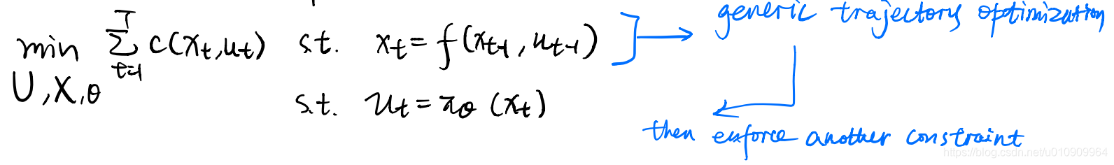
We again come up with a constrained optimization problem, but enforcing the trajectory optimization objective with a new constraint that the policy gives the same actions as our optimal control.

As a digression for Augmented Lagragian, It goes like this.

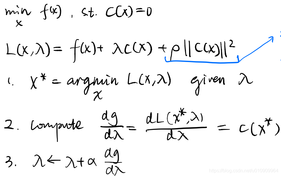
The added term is introduced under such intuition that upon the initial run of the process, the lagragian term does not enforce a strict bound. Here $\rho$ is some constant set at the beginining, so it maintains an emphasis on keeping the constraint satisfied.

So GPS goes like this.

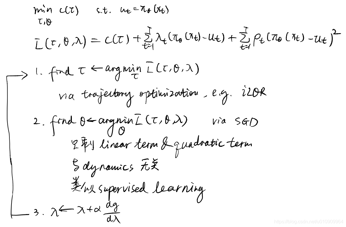
In the first step we do trajectory optimization as normal except that we are guided towards such controls that our policy tends to manage to achieve. This can be seen from the additional two terms for the constraint, where $u_t$ is what the optimal control is planning, and $\pi_\theta(x_t)$ is what current policy tends to propose.

In the second step we are like doing imitation learning for our policy. This is because the gradient of the Lagragian function w.r.t. $\theta$ has nothing to do with the dynamics (intrinsic in the cost term). Left with only the two terms enforcing the constraint, we exactly making our policy to imitate the previous optimal control expert’s demonstrations.

Interpretations for this method are that:

1. this can be viewed as a constrained trajectory optimization problem,
2. we perform imitation learning on the policy with an optimal control expert,
3. the optimal control expert can adapt to the learner (policy), in the sense that while minimizing the intrinsic cost, the controller need also consider the cost (or how hard) the policy can imitate the action.

general scheme

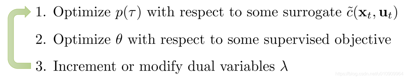
need to choose: 1) form of $\tau$, i.e., deterministic or stochastic, 2) trajectory optimization methods for $\tau$, 3) the proper supervised objective, and 4) the surrogate loss.

Note that the surrogate indeed depends on the supervised objective - It includes the supervised loss as part of its terms. Essentially we use the same objective for step 2 and step 3, just that the first term is independent on $\theta$.

4.3 imitating optimal control with DAgger

In fact, the straight-forward idea of applying imitation learning between an optimal control expert and a parameterized policy should be based on DAgger.

loop {
	1. initialize current state
	2. loop {
		1. run the controller to label the current state, add the state-action pair to D
		2. execute the current policy and interact with the environment, set the state.
	}
	3. fit the policy to D
} until convergence

This approach still corrects the distribution shift, but this time between the trajectory distribution of the controller and the policy.

PLATO
Here is a problem with DAgger. Because we train our policy from scratch, some states can be really awful that definitely do not deserve visiting, and we hope to eliminate the odds of our policy to lead to such states.

initialize state-action dataset D
loop {
	1. train current policy with D
	2. run policy pi_hat and interact with the environment to obtain state data {o_j}
	3. have the states labeled by someone, e.g., expert, to get dataset D_u
	4. aggregate D with D_u
} until convergence

The idea is to introduce another policy to sample from the wanted state distribution, which interpolates between those might well lead to high rewards (which is good) and those occur in current policy (which might well be bad).

Then we formulate this into an optimal control problem, and can solve with iLQR.

4.4 DAgger versus GPS

DAgger has no bounds for the error that the policy fail to match the expert’s behavior. This is problemetic especially in the partial observation case, e.g. the expert at training time has full state while the policy at test time has only partial observations.

GPS allows the expert to adapt to the policy at the cost of having to optimize some additional prescribed cost. This means the solution might be sub-optimal as it takes into consideration the capacity of the policy.

The imitation gets rid of the numerical instability caused by direct backprop into policy (PILCO)

4.5 Dyna: model-free approaches with a learned model

Originally Dyna was proposed in the tabular case:

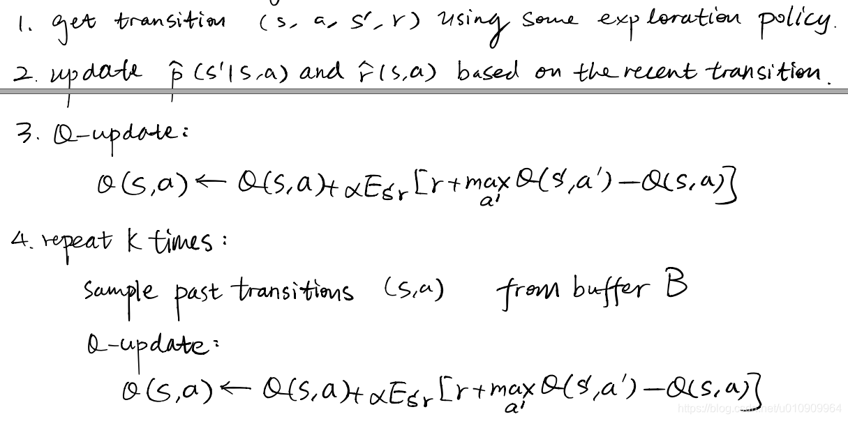
The basic idea is to first learn a model, then use the learned model as a simulator (sample generator) for model-free algorithms to learn a policy, and iterate this process (learn model -> learn policy).

Here is a general recipe for Dyna-Style algorithms.

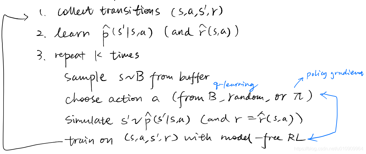
Benefits when compared with pure model-based
When using the learned model as simulator, the samples generated for model-free start from real states obtained from interacting with the environment. We can still view the model-based process as improving a controller with a learned model, just that we now improve via model-free approaches instead of optimal control methods.

Recall that in pure model-based methods, the controller plans with the learned model over a whole trajectory, which involves larger compounding errors. However model-free approaches learns with the model over short rollouts, which involves smaller errors. It’s like the model-free step divides the state space into short rollouts, but manage to see the entirety.

Benefits when compared with pure model-free
more samples are offered to the model-free algorithms, given by the learned model rather than the environment.

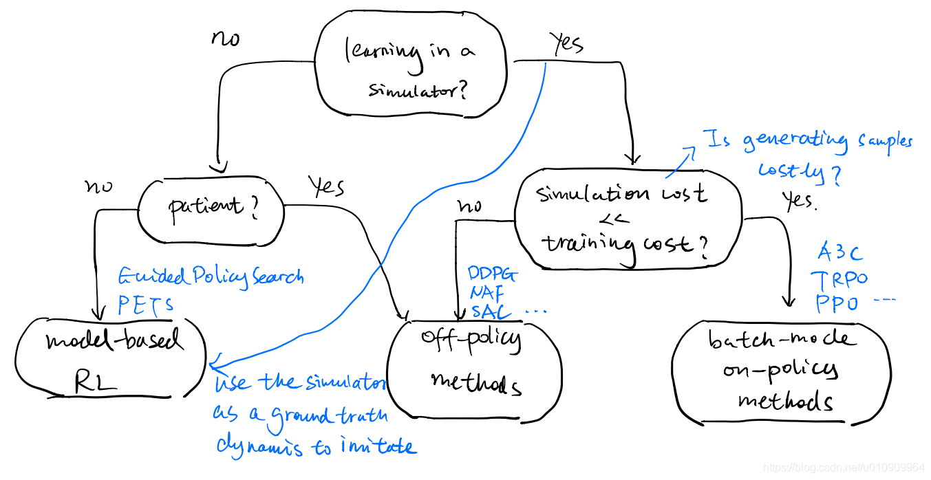
5 How to choose methods

5.1 Sample Efficiency rank

From least efficient to most efficient:

1. gradient-free methods
   evolution strategy, etc.
2. fully online methods
   e.g. A3C
3. (batch-mode online) policy gradient methods: take days
   e.g. TRPO, natural gradient
4. (off-policy) replay buffer value estimation methods: take hours
   e.g. Q-learning, DDPG, NAF, SAC
5. model-based deep RL: take minutes
   e.g. PETS, GPS
6. model-based shallow RL:
   e.g. PILCO (use Gaussian Processes)

5.2 A (rough) road map for RL methods