通过阅读本文,你将:
1.完成ResNet基本的block的构建。
2.将这些blocks组合到一起并完成训练一个基本的网络来完成图片分类任务。
首先加载需要的packages:
import torch
import torch.nn as nn
import torch.optim as optim
from resnets_utils import *

from torch.utils.data import DataLoader, sampler, TensorDataset

import torchvision.datasets as dset

import numpy as np
import h5py
ResNet解决的问题
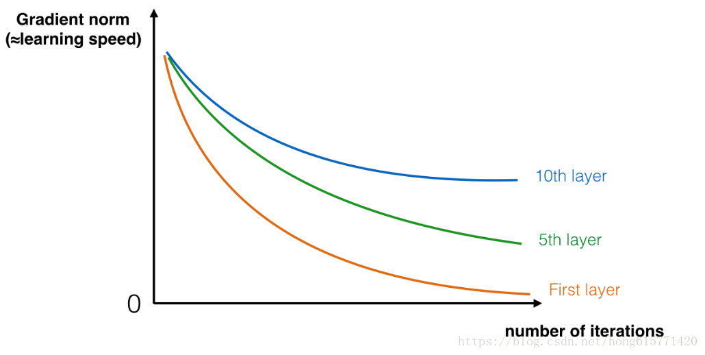
现如今的神经网络深度较大,可达上百层。深度网络的好处就是可以表示非常复杂的函数,它还可以学习到很多不同层次的特征,从边缘检测(此特征在较低的层)到非常复杂的特征(这类特征在更深的层),但是并不是在任何时候使用较深的网络都会得到好效果,一个训练的难点就是会发生梯度消失现象:很深的网络总是会使梯度信号很快消失,这就让梯度下降变得非常缓慢。更需要注意的是,在梯度下降时,当你从最后一层往第一层做反向传播,在每一步你都乘上了权重矩阵,所以梯度可能会以指数倍的下降为0(或者在少数情况下, 会成指数倍的发生梯度爆炸)。
残差网络即解决了上述问题。
构建残差网络
在ResNet中,“shortcut” 和“skip connection”可以让梯度直接传播到前面层。

左边的图即展示了网络的主通道,右边的图在此基础上添加了“shortcut”,通过将这些blocks堆叠,你可以获得很深的网络。
在resnet中主要使用两种block,取决于输入、 输出的尺寸是否相同,你将分别完成他们。
the identity block
identity block是resnet的标准块,当输入的激活值 和输出的激活值
具有相同的维度时使用,下图表示出了这种关系:

上面那条线我们称为“shortcut path”,下面的称为主通道,我们再每一层都进行了conv2d和relu操作,为了加速训练速度,我们还加入了BN层,在本文中 ,你将完成一个更加复杂的block,skip connection将跨过三层隐藏层,如图:

主通道的第一部分:
a.第一个卷积层的卷积核为1*1,步长为1*1,padding为valid,初始化时随机种子为0.
b.第一个BN层标准化 channels axis.
c.然后使用relu激活函数
第二部分:
a.第二个卷积层的卷积核为f*f,步长为1*1,padding为same,随机种子0.
b.第一个BN层标准化 channels axis.
c.然后使用relu激活函数
第三部分:
a.第一个卷积层的卷积核为1*1,步长为1*1,padding为valid,初始化时随机种子为0.
b.第一个BN层标准化 channels axis.
c.然后使用relu激活函数
最后一步:
a.shortcut和input相加
b.然后送入relu激活函数
下面完成identity block的代码:
#identity block doesn't change input sizes and the number of channels. at least in this course.
class identity_block(nn.Module):
    def __init__(self, filters, in_channels):
        super(identity_block, self).__init__()
        F1, F2 = filters
        #First component of the main path
        self.conv2d_1 = nn.Conv2d(in_channels, F1, kernel_size=1) #doesn't change input size
        self.bn_1 = nn.BatchNorm2d(F1)
        self.relu_1 = nn.ReLU()

        #Second component of the main path
        self.conv2d_2 = nn.Conv2d(F1, F2, kernel_size=3, padding=1) #same convolution
        self.bn_2 = nn.BatchNorm2d(F2)
        self.relu_2 = nn.ReLU()

        #Third component of the main path
        #we get back to the original channel size since we assume that the input from the shortcut path and
        #from the main path has the same number of channels when we are using an identity block.
        self.conv2d_3 = nn.Conv2d(F2, in_channels, kernel_size=1) #doesn't change input size
        self.bn_3 = nn.BatchNorm2d(in_channels)
        self.relu_3 = nn.ReLU()

    def forward(self, x):
        x_shortcut = x

        x = self.conv2d_1(x)
        x = self.bn_1(x)
        x = self.relu_1(x)

        x = self.conv2d_2(x)
        x = self.bn_2(x)
        x = self.relu_2(x)

        x = self.conv2d_3(x)
        x = self.bn_3(x)

        x += x_shortcut

        x = self.relu_3(x)

        return x
The convolutional block
You've implemented the ResNet identity block. Next, the ResNet "convolutional block" is the other type of block. You can use this type of block when the input and output dimensions don't match up. The difference with the identity block is that there is a CONV2D layer in the shortcut path:
/images/convblock_kiank.png)
The CONV2D layer in the shortcut path is used to resize the input to a different dimension, so that the dimensions match up in the final addition needed to add the shortcut value back to the main path. (This plays a similar role as the matrix
discussed in lecture.) For example, to reduce the activation dimensions's height and width by a factor of 2, you can use a 1x1 convolution with a stride of 2. The CONV2D layer on the shortcut path does not use any non-linear activation function. Its main role is to just apply a (learned) linear function that reduces the dimension of the input, so that the dimensions match up for the later addition step.
The details of the convolutional block are as follows.
First component of main path:
- The first CONV2D has
filters of shape (1,1) and a stride of (s,s). Its padding is "valid".
- The first BatchNorm is normalizing the channels axis.
- Then apply the ReLU activation function. This has no name and no hyperparameters.
Second component of main path:
- The second CONV2D has
filters of (f,f) and a stride of (1,1). Its padding is "same".
- The second BatchNorm is normalizing the channels axis.
- Then apply the ReLU activation function. This has no name and no hyperparameters.
Third component of main path:
- The third CONV2D has
filters of (1,1) and a stride of (1,1). Its padding is "valid".
- The third BatchNorm is normalizing the channels axis. Note that there is no ReLU activation function in this component.
Shortcut path:
- The CONV2D has
- The BatchNorm is normalizing the channels axis.
Final step:
- The shortcut and the main path values are added together.
- Then apply the ReLU activation function. This has no name and no hyperparameters.
Exercise: Implement the convolutional block. We have implemented the first component of the main path; you should implement the rest. As before, always use 0 as the seed for the random initialization, to ensure consistency with our grader.
- Conv Hint
- BatchNorm Hint
- For the activation, use:
nn.ReLU()
In [46]:
class convolutional_block(nn.Module):
    def __init__(self, filters, s, in_channels):
        super(convolutional_block, self).__init__()

        F1, F2, F3 = filters

        #First component of the main path
        self.conv2d_1 = nn.Conv2d(in_channels, F1, kernel_size=1, stride=s)
        self.bn_1 = nn.BatchNorm2d(F1)
        self.relu_1 = nn.ReLU()

        #Second component of the main path
        self.conv2d_2 = nn.Conv2d(F1, F2, kernel_size=3, padding=1) #3x3 same convolution
        self.bn_2 = nn.BatchNorm2d(F2)
        self.relu_2 = nn.ReLU()

        #Third component of the main path
        self.conv2d_3 = nn.Conv2d(F2, F3, kernel_size=1)
        self.bn_3 = nn.BatchNorm2d(F3)

        #Shortcut path
        #After this, input sizes and the number of channels will match. Because this convolution applies the only
        #transformation that affects the input size, the key point here is stride=s. It's output channels is equal
        #to the number of output channels of the main path.
        self.conv2d_shortcut = nn.Conv2d(in_channels, F3, kernel_size=1, stride=s)
        self.bn_shortcut = nn.BatchNorm2d(F3)

        self.relu_3 = nn.ReLU()

    def forward(self, x):
        x_shortcut = x

        x = self.conv2d_1(x)
        x = self.bn_1(x)
        x = self.relu_1(x)

        x = self.conv2d_2(x)
        x = self.bn_2(x)
        x = self.relu_2(x)

        x = self.conv2d_3(x)
        x = self.bn_3(x)

        x_shortcut = self.conv2d_shortcut(x_shortcut)
        x_shortcut = self.bn_shortcut(x_shortcut)

        x += x_shortcut
        x = self.relu_3(x)

        return x
In [47]:
class Flatten(nn.Module):
    def forward(self, x):
        N, C, H, W = x.size()
        return x.view(N, -1)
In [48]:
num_classes = 6
device = torch.device('cuda:0' if torch.cuda.is_available() else 'cpu')
3 - Building your first ResNet model (50 layers)
You now have the necessary blocks to build a very deep ResNet. The following figure describes in detail the architecture of this neural network. "ID BLOCK" in the diagram stands for "Identity block," and "ID BLOCK x3" means you should stack 3 identity blocks together.
/images/resnet_kiank.png)
The details of this ResNet-50 model are:
- Zero-padding pads the input with a pad of (3,3)
- Stage 1:
- The 2D Convolution has 64 filters of shape (7,7) and uses a stride of (2,2).
- BatchNorm is applied to the channels axis of the input.
- MaxPooling uses a (3,3) window and a (2,2) stride.
- Stage 2:
- The convolutional block uses three set of filters of size [64,64,256], "f" is 3, "s" is 1.
- The 2 identity blocks use three set of filters of size [64,64,256], "f" is 3.
- Stage 3:
- The convolutional block uses three set of filters of size [128,128,512], "f" is 3, "s" is 2.
- The 3 identity blocks use three set of filters of size [128,128,512], "f" is 3.
- Stage 4:
- The convolutional block uses three set of filters of size [256, 256, 1024], "f" is 3, "s" is 2.
- The 5 identity blocks use three set of filters of size [256, 256, 1024], "f" is 3.
- Stage 5:
- The convolutional block uses three set of filters of size [512, 512, 2048], "f" is 3, "s" is 2.
- The 2 identity blocks use three set of filters of size [512, 512, 2048], "f" is 3.
- The 2D Average Pooling uses a window of shape (2,2).
- The flatten doesn't have any hyperparameters.
- The Fully Connected (Dense) layer reduces its input to the number of classes using a softmax activation.
Exercise: Implement the ResNet with 50 layers described in the figure above. We have implemented Stages 1 and 2. Please implement the rest. (The syntax for implementing Stages 3-5 should be quite similar to that of Stage 2.) Make sure you follow the naming convention in the text above.
In [49]:
ResNet50 = nn.Sequential(
    nn.ConstantPad2d(3, 0),
    #---
    #Stage 1
    nn.Conv2d(3, 64, kernel_size=7, stride=2),
    nn.BatchNorm2d(64),
    nn.MaxPool2d(kernel_size=3, stride=2),
    #Stage 2
    convolutional_block([64, 64, 256], s=1, in_channels=64),
    identity_block([64, 64], in_channels=256),
    identity_block([64, 64], in_channels=256),
    #Stage 3
    convolutional_block([128, 128, 512], s=2, in_channels=256),
    identity_block([128, 128], in_channels=512),
    identity_block([128, 128], in_channels=512),
    identity_block([128, 128], in_channels=512),
    #Stage 4
    convolutional_block([256, 256, 1024], s=2, in_channels=512),
    identity_block([256, 256], in_channels=1024),
    identity_block([256, 256], in_channels=1024),
    identity_block([256, 256], in_channels=1024),
    identity_block([256, 256], in_channels=1024),
    identity_block([256, 256], in_channels=1024),
    #Stage 5
    convolutional_block([512, 512, 2048], s=2, in_channels=1024),
    identity_block([512, 512], in_channels=2048),
    identity_block([512, 512], in_channels=2048),
    #---
    nn.AvgPool2d(kernel_size=2), #outputs 1x1x2048
    Flatten(),
    nn.Linear(2048, num_classes)
).to(device)
In [50]:
loss_fn = nn.CrossEntropyLoss()
optimizer = optim.Adam(ResNet50.parameters(), lr=1e-3)
The model is now ready to be trained. The only thing you need is a dataset.
Let's load the SIGNS Dataset.
/images/signs_data_kiank.png)
In [51]:
X_train_orig, Y_train, X_test_orig, Y_test, classes = load_dataset()

#swap axes to make them usable by PyTorch
X_train_orig = np.transpose(X_train_orig, (0, 3, 1, 2))
X_test_orig = np.transpose(X_test_orig, (0, 3, 1, 2))

Y_train = Y_train.ravel()
Y_test = Y_test.ravel()

# Normalize image vectors
X_train = X_train_orig/255.
X_test = X_test_orig/255.

print ("number of training examples = " + str(X_train.shape[0]))
print ("number of test examples = " + str(X_test.shape[0]))
print ("X_train shape: " + str(X_train.shape))
print ("Y_train shape: " + str(Y_train.shape))
print ("X_test shape: " + str(X_test.shape))
print ("Y_test shape: " + str(Y_test.shape))
number of training examples = 1080
number of test examples = 120
X_train shape: (1080, 3, 64, 64)
Y_train shape: (1080,)
X_test shape: (120, 3, 64, 64)
Y_test shape: (120,)
In [52]:
num_train = 1080
num_test = 120
X_train_tensor = torch.tensor(X_train, dtype=torch.float32)
Y_train_tensor = torch.tensor(Y_train, dtype=torch.long)

X_test_tensor = torch.tensor(X_test, dtype=torch.float32)
Y_test_tensor = torch.tensor(Y_test, dtype=torch.long)


train_dataset = TensorDataset(X_train_tensor, Y_train_tensor)
test_dataset = TensorDataset(X_test_tensor, Y_test_tensor)
In [53]:
loader_train = DataLoader(train_dataset, batch_size=32, shuffle=True)
loader_test = DataLoader(test_dataset, batch_size=32, shuffle=True)
In [63]:
def get_accuracy(model, loader_test):
    model.eval()
    num_samples, num_correct = 0, 0
    with torch.no_grad():
        for x, y in loader_test:
            x, y = x.to(device), y.to(device)
            output = model(x)
            _, y_pred = output.data.max(1)
            num_correct += (y_pred == y).sum().item()
            num_samples += x.size(0)

    return num_correct/num_samples

def train(model, loss_fn, optimizer, loader_train, loader_test, epochs=1):
    for epoch in range(epochs):
        model.train()
        for i, (x, y) in enumerate(loader_train):
            x, y = x.to(device), y.to(device)
            y_pred = model(x)

            optimizer.zero_grad()
            loss = loss_fn(y_pred, y)
            loss.backward()

            optimizer.step()
        acc = get_accuracy(model, loader_test)
        print(f"Epoch: {epoch+1} | Loss: {loss.item()} | Test accuracy: {acc}")
In [64]:
train(ResNet50, loss_fn, optimizer, loader_train, loader_test, epochs=3)
Epoch: 1 | Loss: 0.028033534064888954 | Test accuracy: 0.9666666666666667
Epoch: 2 | Loss: 0.05617906525731087 | Test accuracy: 0.9833333333333333
Epoch: 3 | Loss: 0.004207571502774954 | Test accuracy: 0.9666666666666667