机器学习--手写数字识别（KNN、决策树）

KNN 及决策树算法为监督学习中的两种简单算法。

KNN

KNN算法（邻近算法）的核心思想是如果一个样本在特征空间中的k个最相邻的样本中的大多数属于某一个类别，则该样本也属于这个类别，并具有这个类别上样本的特性。
欧式距离的计算公式:

假设每个样本有两个特征值，如 A ：（a1，b1）B：（a2，b2）则AB的欧式距离为

$d=\sqrt{(a1-a2)^2 +(b1-b2)^2}$

例如：根据消费分配来预测性格

在这里插入图片描述

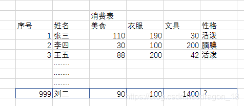
已知张三美食消费为110、衣服消费为190、文具消费为30，张三的性格为活泼。…
根据前3个样本我们算出欧式距离

$d=\sqrt{(110-90)^2+(190-100)^2+(140-30)^2}=143$
$d=\sqrt{(90-30)^2+(100-100)^2+(200-140)^2}=26$
$d=\sqrt{(90-88)^2+(200-100)^2+(140-24)^2}=153$
…

寻找d的最近邻居为143和153，推测出刘二的性格为活泼

决策树

决策树是一种树形结构，其中每个内部节点表示一个属性上的测试，每个分支代表一个测试输出，每个叶节点代表一种类别。

每个决策树都表述了一种树型结构，它由它的分支来对该类型的对象依靠属性进行分类。每个决策树可以依靠对源数据库的分割进行数据测试。这个过程可以递归式的对树进行修剪。当不能再进行分割或一个单独的类可以被应用于某一分支时，递归过程就完成了。

实例

%matplotlib inline

import numpy as np
import matplotlib.pyplot as plt
from sklearn.neighbors import KNeighborsClassifier
from sklearn.tree import DecisionTreeClassifier
from sklearn.linear_model import LogisticRegression
from IPython.display import display

X = []
y = []

for i in range(0,10):
    for j in range(1,701):
        digit = plt.imread('./database/%d/1 (%d).bmp'%(i,j))
        X.append(digit)
        y.append(i)
  
X = np.array(X)
y = np.array(y)
X.shape

index = np.random.randint(0,7000,size=1)[0]
digit = X[index]
plt.figure(figsize=(1,1))
plt.imshow(digit,cmap='gray')
print("true：%d"%(y[index]))

from sklearn.model_selection import train_test_split
X_train,X_test,y_train,y_test = train_test_split(X,y,test_size=0.1)

X_train.shape

knn = KNeighborsClassifier(n_neighbors=5)
knn.fit(X_train.reshape([6300,28*28]),y_train)
knn.score(X_test.reshape([-1,28*28]),y_test)


y_ = knn.predict(X_test.reshape([-1,28*28]))
display(y_[:20],y_test[:20])

X.reshape(7000,-1).shape

#KNN算法实现预测
plt.figure(figsize=(10*1,10*1.5))
for i in range(100):
    axes = plt.subplot(10,10,i+1)
    axes.imshow(X_test[i],cmap='gray')
    t = y_test[i]
    p = y_[i]
    axes.set_title('True:%d\nPred:%d'%(t,p))
    axes.axis('off')
    
#决策树实现预测
##深度为50

plt.figure(figsize=(10*1,10*1.5))
for i in range(100):
    axes = plt.subplot(10,10,i+1)
    axes.imshow(X_test[i],cmap='gray')
    t = y_test[i]
    p = y_[i]
    axes.set_title('True:%d\nPred:%d'%(t,p))
    axes.axis('off')

tree = DecisionTreeClassifier(max_depth=50)

tree.fit(X_train.reshape(6300,-1),y_train)

y_ = tree.predict(X_test.reshape([-1,28*28]))
tree.score(X_test.reshape([-1,28*28]),y_test)

##深度为150

plt.figure(figsize=(10*1,10*1.5))

for i in range(100):
    axes = plt.subplot(10,10,i+1)
    axes.imshow(X_test[i],cmap='gray')
    t = y_test[i]
    p = y_[i]
    axes.set_title('True:%d\nPred:%d'%(t,p))  
    axes.axis('off')


tree = DecisionTreeClassifier(max_depth=150)
tree.fit(X_train.reshape(6300,-1),y_train)
y_ = tree.predict(X_test.reshape([-1,28*28]))
tree.score(X_test.reshape([-1,28*28]),y_test)

机器学习--手写数字识别（KNN、决策树）

KNN

决策树

实例

猜你喜欢