lattice绘图工具

library(lattice)
data1 <- data.frame(x=seq(0,14),y=seq(3,17),z=rep(c("a","b","c"),times=5))
xyplot(y~x,data = data1)

参数	含义
grid.pars	网格图形参数
fontsize	用于文本和符号两个组件(每个组件都是数字标量)的列表
clip	面板和条带两个组件的列表(每个组件都有一个字符串，“开”或“关”)

show.settings()

lattice包通过颜色区分不同组别而不是形状。
xyplot(y~x,groups = z,data = data1)
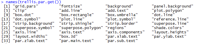
mysettings <- trellis.par.get()
mysettings$superpose.symbol$col <-"black"
mysettings$superpose.symbol$pch <-1:10
trellis.par.set(mysettings)
xyplot(y~x,groups = z,data = data1)

条件变量
graph_function(formula|v,data=,options)
如果条件变量为连续型，需要转为离散型

xyplot(y~x|z,data = data1,layout=c(3,1))

面板函数

mypanel <- function(...){
  panel.abline(a=1,b=1)
  panel.xyplot(...)
}
xyplot(y~x|z,data = data1,layout=c(3,1),panel = mypanel)

分组变量
将不同水平的变量叠加到一起

densityplot(~mpg,data = mtcars,lty=1:2,col=1:2,lwd=2,
            groups = factor(am),
            main=list("MPG分布",cex=1.5),
            xlab = "英里/加仑",
            key=list(column=2,space="bottom",
                     title="类型(0=自动，1=手动)",
                     text=list(levels(factor(mtcars$am))),
                     lines=list(lty=1:2,col=1:2,lwd=2)))

页面摆放
借助plot函数的splite和position

graph1 <- xyplot(mpg~wt,data = mtcars,xlab = "重量",ylab = "英里/加仑")
displacement <- equal.count(mtcars$disp,number=3,overlap=0)
graph2 <- xyplot(mpg~wt|displacement,data= mtcars,layout=c(3,1),
                 xlab = "重量",ylab = "英里/加仑")
plot(graph1,split = c(1,1,2,1))
plot(graph2,split = c(2,1,2,1),newpage = FALSE)

plot(graph1,position = c(0,0,0.5,1))      #图形左下、右上坐标
plot(graph2,position = c(0.6,0.3,1,1),newpage = FALSE)

lattice包绘图函数的常用参数

参数	含义
x	要绘制的对象
data	x为表达式时，动用一个数据框
allow.multiple	对于Y1+Y2X/Z,TRUE时重叠绘制Y1X和Y2X，FALSE时绘制Y1+Y2X
outer	FALSE绘制叠加，TRUE不在一个面板显示
box.ratio	内部矩形长宽比
horizontal	水平或者垂直
panel	面板函数
aspect	不同面板的宽高比
groups
auto.keys	添加分组变量的图例符号
prepanel
strip
xlab,ylab
scales
subscripts
subset
xlim,ylim
drop.unused.levels
default.scales
options

barchart

trellis.par.get("axis.text")
trellis.par.set(list(axis.text = list(cex=1)))
barchart(Titanic,layout=c(4,1),auto.key=TRUE)

barchart(Titanic,layout=c(4,1),auto.key=TRUE,scales = list(x="free"))

barchart(Sex~Freq|Class+Age,data = as.data.frame(Titanic),groups=Survived,
         stack=TRUE,layout=c(8,1),auto.key=TRUE,scales=list(x="free"))

barchart(Sex~Freq|Class+Age,data = as.data.frame(Titanic),groups=Survived,
         stack=TRUE,layout=c(8,1),auto.key=list(title="Survived",columns=2),scales=list(x="free"))

点图

dotplot(VADeaths,pch=1:4,col=1:4,main=list("死亡率",cex=1.5),
        xlab="比率/千人",
        key=list(column=4,text=list(colnames(VADeaths)),points=list(pch=1:4,col=1:4)))

dotplot(VADeaths,groups = FALSE,layout=c(1,4),aspect=0.5,origin=0,type=c(“p”,“h”))

直方图
histogram(x,
data,
allow.multiple, outer = TRUE,
auto.key = FALSE,
aspect = “fill”,
panel = lattice.getOption(“panel.histogram”),
prepanel, scales, strip, groups,
xlab, xlim, ylab, ylim,
type = c(“percent”, “count”, “density”),
nint = if (is.factor(x)) nlevels(x)
else round(log2(length(x)) + 1),
endpoints = extend.limits(range(as.numeric(x),
finite = TRUE), prop = 0.04),
breaks,
equal.widths = TRUE,
drop.unused.levels =
lattice.getOption(“drop.unused.levels”),
…,
lattice.options = NULL,
default.scales = list(),
default.prepanel =
lattice.getOption(“prepanel.default.histogram”),
subscripts,
subset)
核密度图
densityplot(x,
data,
allow.multiple = is.null(groups) || outer,
outer = !is.null(groups),
auto.key = FALSE,
aspect = “fill”,
panel = lattice.getOption(“panel.densityplot”),
prepanel, scales, strip, groups, weights,
xlab, xlim, ylab, ylim,
bw, adjust, kernel, window, width, give.Rkern,
n = 512, from, to, cut, na.rm,
drop.unused.levels =
lattice.getOption(“drop.unused.levels”),
…,
lattice.options = NULL,
default.scales = list(),
default.prepanel =
lattice.getOption(“prepanel.default.densityplot”),
subscripts,
subset)
带状图
panel.stripplot(x, y, jitter.data = FALSE,
factor = 0.5, amount = NULL,
horizontal = TRUE, groups = NULL,
…,
identifier = “stripplot”)
Q-Q图
根据理论分布绘制样本的分位数-分位数图
qqmath(x,
data,
allow.multiple = is.null(groups) || outer,
outer = !is.null(groups),
distribution = qnorm,
f.value = NULL,
auto.key = FALSE,
aspect = “fill”,
panel = lattice.getOption(“panel.qqmath”),
prepanel = NULL,
scales, strip, groups,
xlab, xlim, ylab, ylim,
drop.unused.levels = lattice.getOption(“drop.unused.levels”),
…,
lattice.options = NULL,
default.scales = list(),
default.prepanel = lattice.getOption(“prepanel.default.qqmath”),
subscripts,
subset)
箱型图
bwplot(x,
data,
allow.multiple = is.null(groups) || outer,
outer = FALSE,
auto.key = FALSE,
aspect = “fill”,
panel = lattice.getOption(“panel.bwplot”),
prepanel = NULL,
scales = list(),
strip = TRUE,
groups = NULL,
xlab,
xlim,
ylab,
ylim,
box.ratio = 1,
horizontal = NULL,
drop.unused.levels = lattice.getOption(“drop.unused.levels”),
…,
lattice.options = NULL,
default.scales,
default.prepanel = lattice.getOption(“prepanel.default.bwplot”),
subscripts = !is.null(groups),
subset = TRUE)
散点图矩阵

splom(mtcars[c(1,3:7)],groups = mtcars$cyl,
      pscales = 0 ,pch=1:3,col=1:3,
      varnames = c("M","D","G","R","W","1/4"),
      key=list(columns=3,title="数值",text=list(levels(factor(mtcars$cyl))),
               points=list(pch=1:3,col=1:3)))

三维水平图

data(Cars93,package = "MASS") 
cor_car93 <- cor(Cars93[,!sapply(Cars93,is.factor)],use = "pair")
levelplot(cor_car93,scales=list(x=list(rot=90)))

三维等高线图

contourplot(volcano,cuts=20,label=FALSE)

三维散点图

parset <- list(axis.line = list(col="transparent"),clip=list(panel="off"))
cloud(Sepal.Length~Petal.Length*Petal.Width,data = iris,
      cex=.8,pch=1:3,col=c("blue","green","red"),
      groups = Species,screen=list(z=20,x=-70,y=0),
      par.settings=parset,scales = list(col="black"),
      key=list(title="种类",
      column=3,
      space="bottom",
      text=list(levels(iris$Species)),
      points=list(pch=1:3,col=c("blue","green","red"))))

三维曲面图

wireframe(volcano,shade=TRUE,aspect = c(56/90,0.4),
          light.source=c(10,0,10))